Design and Performance of a 1 Meter Scale Horizontal Axis Wind Turbine Model

(1)

University of New Hampshire

University of New Hampshire Scholars' Repository

Master's Theses and Capstones Student Scholarship

Summer 2018

Design and Performance of a 1 Meter Scale

Horizontal Axis Wind Turbine Model

Samuel Babineau Cole

University of New Hampshire, Durham

Follow this and additional works at:https://scholars.unh.edu/thesis

This Thesis is brought to you for free and open access by the Student Scholarship at University of New Hampshire Scholars' Repository. It has been accepted for inclusion in Master's Theses and Capstones by an authorized administrator of University of New Hampshire Scholars' Repository. For more information, please [email protected].

Recommended Citation

Cole, Samuel Babineau, "Design and Performance of a 1 Meter Scale Horizontal Axis Wind Turbine Model" (2018).Master's Theses and Capstones. 1208.

(2)

DESIGN AND PERFORMANCE OF A 1 METER SCALE HORIZONTAL AXIS WIND TURBINE MODEL

BY

SAMUEL BABINEAU COLE

BS, Mechanical Engineering, University of New Hampshire, New Hampshire , 2016

DISSERTATION

Submitted to the University of New Hampshire in Partial Fulfillment of

the Requirements for the Degree of

Master of Science

in

Mechanical Engineering

(3)

(4)

This thesis has been examined and approved in partial fulfillment of the requirements for the degree of Master of Science in Mechanical Engineering by:

Thesis Director, Martin Wosnik,

Associate Professor of Mechanical Engineering

Barry Fussell,

Professor of Mechanical Engineering

Chris White,

Associate Professor of Mechanical Engineering

Date: May 31, 2018

(5)

(6)

ACKNOWLEDGMENTS

I would like to thank my commitee members, Martin Wosnik, Barry Fussell and Chris White,

for their assistance and guidance throughout this process. I would also like to acknowledge Scott

Campbell for his guidance in fabricating the turbine, and James Abare for his assistance with

the electronics and LabVIEW. Also, support by the National Science Foundation, CBET grant

1150797, Principal Investigator Martin Wosnik, is gratefully acknowledged. Additionally, a huge

thank you goes out to Jim Dreher and the Durham Boat Company who, along with the assistance

of Nick Andrade, made the fabrication of the blades possible. Gavin Hess was instrumental in the

blade and rotor design. I am so grateful for his friendship and support. Lastly, a huge thank you to

(7)

NOMENCLATURE

λ Tip Speed Ratio

Ω Rotor Rotational Velocity

θp Section Pitch Angle

θT Section Twist Angle

θp,0 Blade Pitch Angle

ϕ Angle of Relative Wind

AOA, α Angle of Attack

BEM Blade Element Momentum

Cd Coefficient of Drag

Cl Coefficient of Lift

Cp Power Coefficient

Ct Thrust Coefficient

FD Force of Drag

FL Force of Lift

F P F Flow Physics Facility

HAW T Horizontal Axis Wind Turbine

R Turbine Radius

U Freestream Wind Velocity

Urel Relative Wind Velocity

(11)

LIST OF TABLES

Table Page

1.1 Overview of a selection of similarly sized scale model wind turbines used for

experiments in large wind tunnels. . . 5

2.1 Model Turbine Scaling Factors . . . 15

2.2 Model Turbine Scaled Parameters . . . 16

4.1 Frequency simulation results for the three tower designs. Blade rotational frequency at peak operating condition from performance testing is 119.4

rad/sec. . . 52

(12)

LIST OF FIGURES

Figure Page

1.1 The NTNU 0.9m diameter wind turbine within the test section (2m x 3m cross

section) of the NTNU wind tunnel testing facility [5]. . . 6

1.2 An array of the TUM G1 turbines on a jig to examine offshore turbine array performance in close spacing when subjected to wave-like conditions, shown in the Politecnico di Milano wind tunnel [2]. . . 7

1.3 The 1 meter research wind turbine (G1) used in studying wind turbine array supervisory control and farm optimization facility [2]. . . 8

1.4 The MoWiTO 1.8m diameter model turbine shown in the WindLab at University Oldenburg in front of the active grid for controlling inflow turbulence [3]. . . 9

2.1 The FPF at the University of New Hampshire. A section view. Test section is 72 m (length) x 6 m (width) x 2.7 m (height). . . 12

3.1 The actuator disk model of a wind turbine. Figure adapted from Manwel et al.[22]. . . 18

3.2 Theoretical maximumCp as a function of tip speed ratio, with and without wake rotation. Figure from Manwell et al. [22]. . . 21

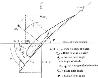
3.3 The blade geometry and variable definitions for use in blade element momentum theory. Figure from Manwell et al. [22]. . . 22

3.4 SG6040 Polar comparison of XFOIL and empirical data from [16]. . . 27

3.5 SG6042 Polar comparison of XFOIL and Selig’s empirical data from [16]. . . 28

3.6 Effect of adjusting XFOIL turbulence parameter, Ncrit . . . 29

3.7 "Root" airfoilCl/Cdcomparisoin at Re = 150k . . . 30

3.8 "Tip" airfoilCl/Cdcomparisoin at Re = 210k . . . 31

(13)

3.10 2-D Profile of the selected NREL S801 airfoil . . . 34

3.11 The blade geometries for the 1.35x (left) and 1.7x (right) chord scaling. Note the twist distribution was un-adjusted. . . 35

3.12 Estimated performance from QBlade BEM versus blade chord scale. . . 35

4.1 The main components of modern wind turbines, from [22]. . . 37

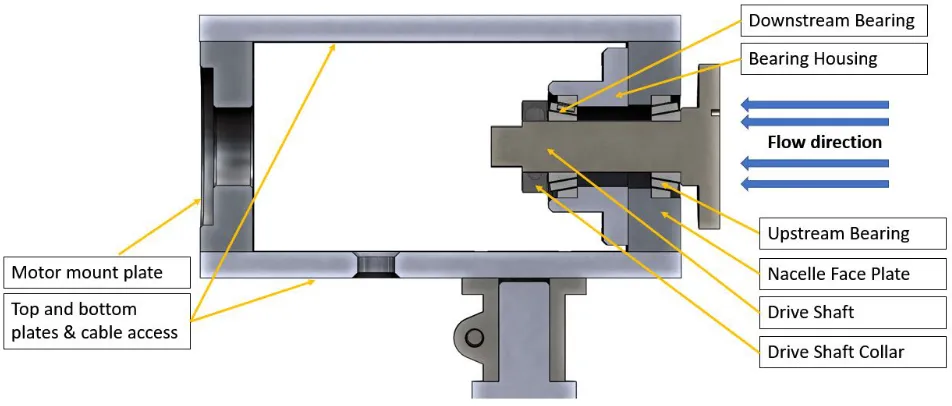
4.2 A section view of the driveshaft support bearings. Flow from right to left. . . 38

4.3 The downstream tapered bearing housing. . . 39

4.4 Detailed view of the turbine drive train. . . 40

4.5 The completed nacelle assembly. In this image the blades are not yet glued and pinned to the roots and pitch control mechanisms. . . 41

4.6 The stages of driveshaft fabrication. The drive shafts (shown left to right) are a 3D printed rapid prototype, the drive shaft prior to parting off and drilling/reaming and, to the far right, the completed part. . . 42

4.7 The rotor hub assembly. This figure shows the hub and three root housings. Also shown are the three NewPort 127 thread per inch blade pitch adjustement screws. . . 42

4.8 Exploded view of the pitch control assembly. Each blade is connected to one of these assemblies. . . 43

4.9 A view of the pitch adjustment assemblies and blades attached to the hub/drive shaft. . . 43

4.10 The solid model design of the mold. . . 45

4.11 The mandrel inserted into the mold. . . 46

4.12 The carbon fiber sheets pressed in one half of the blade mold. . . 46

4.13 The 1.7x(top) and 1.35x(bottom) chord scaled blades after removal from the mold. . . 47

(14)

4.15 Exploded view of the jig used to mount the alignment laser to the blades. From top to bottom, the 4-40 tightening screws, the jig top half and laser mount (blue), a representation of the blade section to which the jig attaches (orange), the jig bottom half (green) and the brass tensioning knobs (to tighten down the jig). . . 48

4.16 The laser jig used to glue the root into the blades with the keyway in the correct location. A similar process was used during testing to set blade pitch angle of

the blades once installed on the turbine. That is shown later in 7. . . 49

4.17 Freestream (left) and boundary layer (right) test configurations. Hub heights are 1.35 and 0.71 meters for the free stream and boundary layer testing

respectively. . . 50

4.18 Plot of the mesh and load case for the selected tower. The tower shown in this image is representative of the tests performed on the one, two, and three tiered tower designs. The base is fixed in translation and rotation and the applied

load is 100N (2x the estimated thrust) in the downstream direction. . . 51

4.19 The tower design selected for use on the UNH 1m HAWT. Note that the 24 inch bottom section can be removed so the hub height will be low enough to test

the turbine in a boundary layer. . . 53

4.20 The force balance. . . 54

4.21 Overview of the UNH 1m HAWT design. . . 55

4.22 A schematic outlining the force balance calibration. The two load cases shown

calibrate for tower only testing (left) and full turbine loading (right). . . 56

4.23 Calibration curve for the full turbine load case. Curve was generated by loading and unloading the force balance from the resultant location of loading for full

turbine testing. . . 57

4.24 Calibration curve for the tower only load case. Note the considerable hysteresis between the ’loading’ and ’unloading’. The difference between some of these points is larger than the uncertainty of the load cell, therefore there is some

stiction in the force balance ball bearing carriages. . . 57

4.25 The calibration curve for the power lost to the driveshaft support bearings, based

on the rotational rate of the turbine. . . 58

5.1 The electronics enclosure, shown in the FPF test section. . . 61

(15)

5.3 Torque-speed curve for the Parker Hannifin BE344J servo motor used to control

speed and generate power on the 1m turbine. . . 65

5.4 A basic PID control block diagram [12]. . . 66

5.5 The LabVIEW turbine monitor and control interface. . . 70

6.1 Experimental test setup. A birds-eye view. Depicts the experiments in free stream. Turbine location: FPF top view (top) and side view (bottom) with the model turbine installed in the center of the test section (free stream) at x=5m

downstream of test section inlet. Flow is left to right. (Note that the locations of floating element drag plates and optical quality windows are also shown−

they will not be used in this project.) . . . 71

6.2 Experimental test setup. The turbine is shown here at 8 meters from the tunnel’s

inlet. In the background the wake measurement traverse is shown. . . 72

6.3 The measured incoming mean flow speeds at the FPF, measured 5m from the inlet. It is shown in this figure to not be the uniform inflow. This yields lower available power than a uniform inflow would have, causing performance of the turbine to be underestimated slightly in this work. The effects of a velocity gradient on a turbine rotor is not fully understood at this time. Figure adapted

from [33]. . . 73

7.1 An example plot for Power vs. Time from the turbine, tested at a free-stream wind speed of 9.5 m/s. For this test tip speed ratio was varied from 4 to 8. . . 77

7.2 An example plot for Thrust vs Time. The thrust versus time for the same test as

shown in the previous figure. Tip speed ratio was varied from 4 to 8. . . 78

7.3 Turbine performance for a range of wind speeds, and tip speed ratios ranging from 4 to 8. Peak values ofCp = 0.34andCT = 1.05are shown atλ= 6.1 . . . 80 7.4 Turbine performance for a range of wind speeds, and tip speed ratios ranging

from 4 to 8. Reynolds number independent performance is shown above

7.5m/s. . . 81 7.5 Turbine performance curves showing the errorbars for eachCpandCtpoint. . . 82

7.6 Comparison of the measured turbine power coefficient and the power coefficients

estimated using the QBlade BEM code. . . 83

7.7 A schematic (top view, looking down the tower) showing where the flow tripping strips are attached to the tower sections. Strips were applied in this

(16)

7.8 A plot showing the change in drag coeffience with the flow tripping strips

installed. The emerical data was taken from Fox et al. and all calculations are

based on averade tower diameter. . . 85

7.9 Schematic explaining laser alignment of blade pitch angle. . . 86

7.10 The laser alignment of blade pitch angle within the FPF test section. . . 86

7.11 The mean power from each tip speed ratio set point for the pitch angle tests. Note how at±1degree of pitch angle the performance declines in comparison to

the zero pitch angle performance. . . 87

7.12 TheCp curves for the pitch angle tests. Again, as shown in the Figure 7.11,±1

degree of blade pitch angle yields lesser performance compared to the zero

(17)

ABSTRACT

Design and Performance of a 1 Meter Scale Horizontal Axis Wind Turbine

Model

by

Samuel Babineau Cole

University of New Hampshire, September, 2018

A research wind turbine of one meter diameter was designed for the use in the UNH Flow

Physics Facility (FPF), a large flow physics quality boundary layer wind tunnel. The turbine

de-sign was carried out as an aero-servo model of the NREL 5MW reference turbine, with some

modifications. The turbine is used to obtain data for multiscale wake model verification and

vali-dation, including wake data over long distances downstream. Blockage in the FPF test section is

4.8%based on rotor swept area.

The rotor was designed using blade element momentum theory based on the S801 airfoil. The

optimal blade chord was scaled by 1.35 and 1.7 to raise the chord based Reynolds number. This

was done to achieve Reynolds number independent performance. Also, the blade pitch angle can

be precisely adjusted.

The turbine is designed to actively control tip speed ratio, as well as record torque, rotor

rota-tional velocity, and thrust. The tip speed ratio control is achieved with aParker HannifinBE344J

series servo motor and Compax3 drive. A Futek LSB302load cell is used in a single axis force

balance to record thrust and aFutek TRS605rotary torque transducer is used to record torque and

rotational velocity. ANational Instruments USB6211data acquisition board and custom LabVIEW

machine interface was used to manage the signals and implement the control logic.

Turbine performance was examined in the free stream. Reynolds number independent

perfor-mance was shown above wind speeds of 7.5 m/s. Perforperfor-mance of the turbine was characterized

and maximum performance was shown atλ= 6.1withCp ≈0.35andCt≈1.05. The effect blade pitch angle was also examined and it was shown that the peak turbine performance is at a blade

(18)

CHAPTER 1 INTRODUCTION

1.1 Motivation

1_{Increasingly large wind farms, both onshore and offshore, must be designed with flow-physics}

based numerical models, and validation data for these models are needed across a spectrum of

scales. From a flow-physics perspective, there is a need for detailed experimental data for wind

turbine wakes to improve our understanding of wakes and ultimately wind turbine array spacing.

Numerical simulations are generally better suited to explore the turbine array design

parame-ter space than physical models, since physical model studies of large wind turbine arrays at large

model scale would be very expensive. However, since the computing power available today is not

sufficient to conduct simulations of the flow in and around large arrays of turbines with

turbulence-resolving direct numerical simulations (DNS) and fully resolved turbine geometries, models are

needed. The flow field (wind resource, atmospheric boundary layer) is typically modeled using

computational fluid dynamics (CFD) with Reynolds-averaged Navier Stokes (RANS) turbulence

models ([34]) or large eddy simulation (LES) ([38],[37],[36]) and the turbines’ interaction with the

wind energy resource is parameterized, or modeled as well, for example with actuator disk (ADM)

or line models (ALM) ([31], [6], [25], [24]). It should be noted that presently this level of fidelity

in simulations is rarely used in industry by those who are planning wind farm layouts. Very simple

wake models, such as the Jensen (1983) model that represents the wake as an axisymmetric top-hat

profile that spreads and lessens in strength with downstream distance using a decay parameter, are

still used by wind farm designers. However, as more High Performance Computing (HPC)

(19)

ity becomes available, developers will be moving to higher fidelity simulations – initially RANS

and eventually LES. Validation data from scaled experiments will help improve these models and

further validate them to build trust in industry.

Validation data for numerical models are needed across a spectrum of scales: at full scale (in

the MW class), at the "SWiFT"scale (using Vestas V27 turbines, [20]), at large rotor scale in very

large cross section aerodynamic wind tunnels (e.g., NASA Ames [14][29], DNW German-Dutch

[30] [9] wind tunnels) as well as at the "as-large-as-feasible"scale in large atmospheric boundary

layer wind tunnels. Each of these scales allows different types of measurements, and provides

valuable data for model validation.

Full scale wind turbine and wind farm data typically does not have fine-grained flow

informa-tion for inflow and turbine wake, and the boundary condiinforma-tions (wind resource) are highly variable

and cannot be controlled. However, full scale measurements, or correctly predicted energy

pro-duction will ultimately be the arbiter on whether flow-physics based computational engineering

models did a good job in predicting the performance of a real wind farm. Numerical simulations

of wind farms are often "indirectly"validated against turbine power data from the SCADA system,

replicating the spacing of the wind turbines and using the information from the wind farm

meteoro-logical tower for inflow information. Due to increased usage of field-deployable flow measurement

techniques such as LIDAR, increasingly valuable wind farm data and analysis of these data exists.

However, wind farm data is generally treated as proprietary information for commercial wind farms

and not openly available, and it still has the drawback of uncontrolled conditions.

Laboratory experiments with wind turbines, i.e., wind tunnel studies, on the other hand allow

for well-controlled conditions. The downside is that often these studies do not provide information

sufficiently far downstream of the turbine rotor, mostly due to facility size restrictions. There have

been a number of recent studies in large facilities that were conducted specifically to address this,

e.g. the, "MEXICO"experiments in the DNW wind tunnel that studied performance of a large

rotor (by wind tunnel standards) ([30]) or the experiments of Krogstad et al (e.g.,[19]), which used

(20)

The experiments enabled by the scale model turbine described in this paper will achieve similar

Reynolds numbers as in the Krogstad et al. study. However, due to the combination of turbine and

facility sizes, the experiments will be able to move beyond some of the limitations of that study, in

1. that the model turbines will have significantly lower blockage ratio for a turbine of similar

scale to those listed in Table 1.1,

2. that we will be able to obtain wake information much further downstream of the rotor, due

to the size of the UNH Flow Physics Facility, and

3. that we will be able to place turbines within a turbulent boundary layer and also investigate

phenomena such as wake meandering.

Furthermore, there is a need for detailed experimental data for wind turbine wakes to improve

our general understanding of wakes and ultimately wind turbine array spacing. Wind turbine

ar-rays can suffer from a significant overall energy production shortfall, due to wakes generated by

turbines upstream interacting with turbines downstream. Energy production losses due to these

array wake effects, when averaged over a year and all wind directions, typically range from 5% to

over 15% of rated wind farm capacity for on-shore wind farms, depending on wind farm layout

([8]). Array wake effects losses have been measured as high as 20% in large off-shore wind farms

with regularly-spaced wind turbines ([7]).

A good deal about turbine wakes, turbulence intensities, wake energy budgets and wake-wake

interactions remains unknown. While array losses can clearly not be completely avoided as long

as wind turbines are deployed in arrays, the cost of this limited understanding is significant.

1.2 Background

The Department of Energy provided a comprehensive analysis of the status of wind energy in the

United States in 2015. The goal of this initiative was to review the Dept. of Energy’s original

2008 report, 20% Wind by 2030. This re-evaluation was guided by 4 major objectives [21]: (1)

(21)

wind power contributions to the U.S energy profile, (3) quantify cost, benefit and the other impacts

of the continued expansion of U.S. wind energy, and (4) to identify the optimal action items to

continue moving U.S. wind energy forward.

The fourth objective of the Wind Vision report consists of an expansive list of action items that

will aid in improving the status of wind energy in the United States. The work that is presented

here falls under Action Item 2.3: Improve and Validate Advanced Simulation and System Design

Tools. This particular action item is working towards developing and validating a comprehensive

suite of engineering, simulation and physics based tools for the design and analysis of wind plants.

This is imperative in order to reach the goal of 20% Wind by 2030. The validation data sets that

are required are high resolution wind turbine wake and performance data sets from multiple scales.

The scales at which validation data is desired are:

1. Full scale (MW class turbines,D≈100m)

2. "SWiFT" scale (D≈25m)

3. "Large-Rotor" scale (D≈5−10m)

4. "As-Large-As-Feasible scale (D≈1−2m)

Work has been performed at each of the scales listed above, and each comes with its own set

of pros and cons. At the full scale, the turbine wake is the most realistic, however the flow field is

un-controlled and generally not well known. Data sets at the full scale are also generally expensive

to acquire and often not made public. The "SWiFT" scale is named based on a testing done by

the Dept. of Energy using 3 Vestas V27 turbines in an L configuration [20]. These test however

were performed in the field, where the flow conditions are difficult to characterize. There has also

been testing performed at the "Large-Rotor" scale, such as the work performed as NASA Ames

(22)

is where the "As-Large-As-Feasible scale comes in. Testing at this scale is typically performed in

large boundary layer wind tunnels, and due to their small diameter size, wake data can be recorded

many diameters downstream.

The turbine presented in this work is not the first or only research performed on this topic.

Many turbines of a similar scale have been designed and built to examine some of the similar

questions the UNH 1m HAWT will address. The scale at which all of these turbines are working

is the ’as-large-as-feasible’ scale. These are turbines typically on the order of 1-2m diameter, best

tested in large boundary layer wind tunnels.In fact there have been many such turbines designed

with the goal of examining turbine performance and wakes. An overview of these turbines is shown

in Table 1.1.

Institution Diameter TSR Blockage Reynolds Number Reference

NTNU 0.9m 6 12.4% ≈110,000@tip [19]

TUM ’G0.6’ 0.58m 6 5.8% ≈64,000@tip [4]

TUM ’G1’ 1.1m 7 1.4% ≈100,000@tip [11]

TUM ’G2’ 2m 7.5 5.9% ≈60,000@75%chord [10]

MoWiTO 1.8m 7.5 28% ≈100,000@75%chord [4]

UNH 1m HAWT 1m 6 4.8% ≈80,000@75%chord This thesis

Table 1.1: Overview of a selection of similarly sized scale model wind turbines used for experi-ments in large wind tunnels.

*Note: TUM is Technische Universitat Munchen, and NTNU is the Norwegian University of

Science and Technology, and MoWiTO is Model Wind Turbine Oldenburg

The NTNU is the turbine which is most closely related to the work performed here at the

Uni-versity of New Hampshire. The studies performed by Krogstad et al represent a turbine with similar

diameter, blade chord scaling and control authority, to the UNH turbine however the NTNU testing

facility does not allow for measurement very far downstream, and also yields≈ 12.4% blockage. The turbine rotor was designed around the S826 airfoil profile. The nacelle is instrumented to

record torque, angular velocity and thrust. The measured Cp and CT were ≈ 0.45 and ≈ 0.9

(23)

Figure 1.1:The NTNU 0.9m diameter wind turbine within the test section (2m x 3m cross section) of the NTNU wind tunnel testing facility [5].

Recently the NTNU group has expanded their studies to multiple turbines within the flow to

examine turbine-turbine interactions[27].

The TUM series of turbines is also quite similar to Krogstad and UNH in their wind energy

research. This family of turbines ranges in diameter, including a 0.6m, 1m and 2m turbine, labeled

the G0.6, G1, and G2 respectively. These turbines are used for many different types of studies,

ranging from wake dynamics (with the smaller turbines) to control theory (the focus of the G2

turbine). The G2 turbine has also been used to examine turbine loading and fatigue as it is fully

instrumented to determine bending moments on the tower and blades. The G2 rotor is based on

two airfoils, both with turbulators and adjustments to thickness, the WM006 and AH79-100c.

The TUM turbines are also used for examining supervisory control systems, and most recently,

(24)

Figure 1.2: An array of the TUM G1 turbines on a jig to examine offshore turbine array perfor-mance in close spacing when subjected to wave-like conditions, shown in the Politecnico di Milano wind tunnel [2].

The turbine in the TUM family that is most closely related to the UNH 1m HAWT is the TUM

(25)

Figure 1.3: The 1 meter research wind turbine (G1) used in studying wind turbine array supervi-sory control and farm optimization facility [2].

The MoWiTO 1.8 turbine is another example of a turbine of similar scale to the UNH 1m

turbine. The MoWiTO is a 1.8m diameter turbine which operates at maximum performance at a

tip speed ratio of 7.5. This turbine has a maximum power coefficient of≈0.4and atλ= 7.5thrust coefficient is≈ 0.91. The turbine has blade aerodynamics and loads scalable to the NREL 5MW reference turbine. This 1.8m turbine is examined in the WindLab at University Oldenburg. This

tunnel can be operated in an enclosed configuration (test section of dimensions (H x W x L) of 3m

x 3m x 30m), or in a n open configuration in which the flow enters a large space from a 3x3 meter

inlet. This turbine was tested in the open configuration. This testing facility features a large active

grid for controlling inflow conditions. It is a 20 split axis system, driven by 80 servo motors to

allow the turbulence in the inflow to be controlled. The MoWiTO 1.8m turbine has been involved

(26)

Figure 1.4: The MoWiTO 1.8m diameter model turbine shown in the WindLab at University Oldenburg in front of the active grid for controlling inflow turbulence [3].

These turbines all aim to achieve the same goals as the turbine presented here. They are used

in generating validation and verification data sets for high fidelity CFD models. They also aim to

improve the general understanding of turbine wakes.

1.3 Objectives

The UNH 1m horizontal axis wind turbine was designed with a few major objectives in mind.

These objectives were selected such that the data from the turbine will aid in the Department of

Energy’s High-Level Wind Vision Roadmap Actions [21]. The turbine must:

1. generate an axisymmetric wake which is kinematically similar to that of a full scale wind

(27)

2. have a fully defined scaled geometry

3. actively control the tip speed ratio (λ)

4. allow for manual variation of the blade pitch angle.

This turbine will have it’s performance characterized with power and thrust coefficient versus

tip speed ratio plots. It will be used in generating wake model validation data sets.

The objectives for this turbine, along with considerations of cost and manufacturability were

the driving forces behind the design methodology for this turbine. The instruments were selected

to provide the data necessary to characterize the turbine, and in most cases, the form factor of

those instruments, and the status of current wind turbine design, constrained and formulated the

component designs. The rotor, mechanical and electrical design of the turbine are presented in the

(28)

CHAPTER 2 SCALING

The physical scale of the model wind turbine will be determined by the size of the available

wind tunnel and by what is considered an acceptable blockage ratio. Therefore the dicussion of

scaling begins with an examination of the testing facility.

2.1 Testing Facility

The Flow Physics Facility (FPF) is a large turbulent boundary layer wind tunnel with test

section dimensions 72m long x 6m wide x 2.7m high. The ceiling height increases from 2.7m at

the test section entrance to 2.9m at the exit into the downstream plenum to compensate for the

growth of boundary layers on all four walls. The FPF is well suited for this work as it is large

enough to test anO(1m) scale model wind turbine in both the free stream (near the entrance of the test section) as well as within an artificially thickened boundary layer further downstream in

the test section. It is also of sufficient length and cross-section to allow wake measurements many

diameters downstream of the turbine rotor.

The FPF is powered by two 400-horsepower fans, which can draw air through the test section

up to a combined 500,000 cubic feet per minute. The maximum test section free stream velocity

in its present state (FPF Phase 1, open return) is 14 m/s (30 mph).

The size of the wind tunnel test section, and simultaneous consideration of the effect of

block-age (ratio of the rotor swept area to the test section cross sectional area) on the performance of

a wind turbine, set the limit of the geometric scale possible for the model turbine. Sarlak et al.

[28] showed that for a rotating turbine rotor under a uniform inflow condition, power and thrust

(29)

Figure 2.1: The FPF at the University of New Hampshire. A section view. Test section is 72 m (length) x 6 m (width) x 2.7 m (height).

A 1 meter diameter was selected for the model wind turbine, yielding a blockage ratio in the

FPF test section of slightly less than 5% as shown in Equation 2.3.

With the tunnel cross sectional area:

Ac.s,F P F = 6∗2.7 = 16.2m2 (2.1)

and turbine radiusR = D₂ = 0.5m:

Arotor=π(R2) = π(0.52) = 0.785m2 (2.2)

the blockage of the wind turbine within the FPF test section is:

Blockage= Arotor

Ac.s,F P F

(100) = 4.85% (2.3)

2.2 Turbine Scaling

The turbines tested in boundary layer wind tunnels need to be scaled based on a reference

turbine so that the data can be applied to models that will eventually predict performance at the

(30)

To achieve this, the model turbines that are studied aim to operate at the same tip speed ratio so

that the angle of relative wind on the scaled blades is the same as the full scale. By doing this, the

interaction of the rotor with the flow is similar across the scales. This causes the wake generated

by that interaction to be similar between the model and full scale turbine. It should be noted that

the blades are not geometrically scaled, with matching chord lengths or airfoils along the blades.

This has been shown to provide poor performance at the model scale [23] and the geometry for the

full scale accounts for the loading at that scale, which is not necessary in the model testing.

Depending on the geometric scale at which the model turbine is built, the elastic properties and

component natural frequencies may or may not be scaled. An aero-servo-elastic model, such at the

model turbine shown in Campagnolo et al. ([10]) is scaled geometrically, provides the kinematic

similarity dicussed above, but also shares the same control actuation and scales the elasticity of the

full scale reference turbine.

The turbine that is presented in this work is an aero-servo model. This means that the turbine

is designed to generate a kinematically similar wake profile, and is geometrically scaled (length

scale factor of 1:126), however the elasticity is not scaled, and the turbine is designed to be rigid

(deflections are minimized until negligible). This makes the turbine easier to use in numerical

models, but it is also necessary at this scale. In order to scale elastically, the masses would need

to be scaled appropriately. This is impossible at this scale because masses scale by density and the

volume scaling factor, which is the cube of the length scaling factor since the units of volume are

m3_{. The length scale factor is} _{1 : 126}_{, so the masses would scale by}_{1 : 126}3 _{which is far from} possible with current materials and manufacturing capabilities.

The scaling procedure for the model turbine was conducted under the following assumptions.

1. The ratio of material densities between the full scale and the model is assumed in all cases

to be equal to one.

2. The model is assumed rigid, as the masses scale with the cube of the length scale factor

(31)

3. Tip speed ratio will be held constant between the full scale and the model turbine (kinematic

wake similarity).

4. The Mach number of the full scale is low enough (<< 0.3) that the scale factor for wind speed will be the ratio of free stream velocities as the flow is incompressible [10].

2.2.1 Turbine Scaling Constraints

From the blockage ratio evaluation the model turbine rotor diameter was established. The

turbine is being scaled with respect to the NREL reference 5MW turbine defined in [18]. The rotor

diameter of this reference turbine is 126 meters and thus the length scaling factor (Eq.2.4) is set

as the ratio of the model rotor diameter to the full scale turbine rotor diameter. Here forward, the

subscripts ’m’ and ’fs’ denote ’model’ and ’full scale’ respectively.

nl =Dm/Df s = 1/126 (2.4)

From [22] the formulation of tip speed ratioλis as follows, whereΩis the rotational speed of the turbine,Ris the rotor radius andU∞is the free-stream flow speed.

λ= ΩR/U∞ (2.5)

In compliance with assumption 3 the full scale and model scale tip speed ratios were equated.

ΩmRm/U∞,m = Ωf sRf s/U∞f s (2.6)

This shows the rotor speed scales with the time scale divided by the length scale. With the

length scale defined, and the wind speed scale factor (nU = 1) from assumption 4, the rotor speed scaling factor is

nΩ =nU/nl (2.7)

(32)

From [22] the power (neglecting power train efficiency) from a turbine is defined as:

P =Cp0.5ρπR2U∞3 (2.8)

Equation 2.8 shows that the scaling factor for power is dependent on the square of length scale

factor and the cube of the wind speed scale factor. An estimate of power from the scale model

turbine can be found using power scaling factor:

nP =n2ln 3

U (2.9)

Similarly, thrust and torque scaling factors (nT and nQ respectively) were determined. The

model scaling factors are provided in Table 2.1.

Table 2.1: Model Turbine Scaling Factors

Quantity Scaling Factor Relationship Value

Length nl _DDm

f s 1 : 126

Wind Speed nU (

U∞,m

U∞,f s) 1 : 1

Rotor Rot. Speed nΩ _nl1 126 : 1

Power nP (_{Df s}Dm)2(_{U∞,f s}U∞,m)3 1 : 15876

Thrust nT (_{Df s}Dm)2(_{U∞,f s}U∞,m)2 1 : 15876

Torque nQ (_{Df s}Dm)3(_{U∞,f s}U∞,m)2 1 : 20e5

2.2.2 Scale Model Turbine Definition

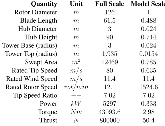
The values fornP,nQ, andnT are dependent on the wind speed in the wind tunnel, so they are

subject to vary from the values provided here. The FPF is capable of running at wind speeds up

to 14 m/sec (above the 5 MW turbine rated wind speed of11.4m/s [18]). In Table 2.1 and Table 2.2 the wind speed scale factor was assumed to be equal to 1. The full scale parameters [18] were

mapped through these scaling factors to give the design values for the model. These are presented

(33)

Table 2.2: Model Turbine Scaled Parameters

Quantity Unit Full Scale Model Scale

Rotor Diameter m 126 1

Blade Length m 61.5 0.488

Hub Diameter m 3 0.024

Hub Height m 90 0.714

Tower Base (radius) m 3 0.024

Tower Top (radius) m 1.935 0.0154

Swept Area m2 ₁₂₄₆₉ ₀_.₇₈₅

Rated Tip Speed m/s 80 0.635

Rated Wind Speed m/s 11.4 11.4

Rated Rotor Speed rot/min 12.1 1524.6

Tip Speed Ratio −− 7.02 7.02

Power kW 5297 0.333

Torque N m 43093.6 2.98

(34)

CHAPTER 3 ROTOR DESIGN

In this chapter the design of the UNH 1m HAWT rotor is examined. This will begin with a

brief overview of the important concepts surrounding the behavior of wind turbine rotors and the

airflow surrounding them. One dimensional momentum theory and airfoil aerodynamics will be

introduced, which will lay the groundwork for examination of rotor performance based on blades

designed by way of Blade Element Momentum (BEM) theory.

3.1 Momentum Theory

No discussion of wind turbine performance is complete without an examination of one dimensional

momentum thoery and the Betz limit [22]. This will be presented here. For more details see

Manwell et al.

A control volume is established surrounding an actuator disk representing the rotor swept area,

where the boundaries of the control volume are defined as the stream-tube boundary. This control

(35)

Figure 3.1: The actuator disk model of a wind turbine. Figure adapted from Manwel et al.[22].

This analysis assumes (i) homogeneous and incompressible flow, (ii) no fricional drag, (iii)

in-finite number of blades, (iv) uniform thrust over rotor area, (v) non-rotating wake (for the moment),

and (vi) ambient static pressure far up and down stream of the rotor plane.

Thrust on the actuator disk can be expressed in two ways. First, from conservation of linear

momentum:

T =U1(ρAU)1−U4(ρAU)4 (3.1)

Then also by expressing thrust as the sum of the forces on either side of the disk:

T = 1

2ρA(U

2

1 −U

2

4) (3.2)

These two representations for thrust can be equated to show that the velocity at the rotor plane

is equal to the average of the upstream and downstream velocities for this model.

By defining an axial inductance factor (a) as the decrease of velocity through the rotor,

normal-ized by the incoming velocity:

a= U1−U2

U1

(36)

U2 =U1(1−a) (3.4)

So as the axial inductance factor increases from zero, the velocity at the rotor decreases,

repre-senting momentum taken from the flow.

Power from the actuator disk can then be shown to be

P = 1

2ρAU

3

14a(1−a) 2

(3.5)

and the non-dimentionalized performance of the turbine is defined as:

Cp =

P 1

2ρAU

3 (3.6)

substituting forP,

Cp = 4a(1−a)2 (3.7)

Maximum possible power can then be found by taking the derivative of 3.7 with respect to a

and setting that equal to 0. This yieldsa = 1/3making the maximum power coefficient possible (known as the Betz limit [22])

Cp,max =

16

27 = 0.593 (3.8)

The model presented thus far does not account for wake rotation, which plays a significant role

in turbine power production. When introduced into the model, the equations change slightly.

When the rotational kinetic energy imparted on the wake by the rotor is considered, the energy

extracted from the flow is less than in the non-rotating case. The assumption of equal pressures far

up and downstream if the angular velocity of the flow stream (ω) is considered small in comparison

(37)

a0 = ω

2Ω (3.9)

then the thrust on a radial annular disk is expressed as:

dT = 4a0(1 +a0)1 2ρΩ

2

r22πrdr (3.10)

Thrust without the rotation considered is based only on the axial inductance factor[22]

dT = 4a(1−a)1

2ρU

2₂_πrdr _(3.11)

Equating 3.10 and 3.11 yields the following equation, which introduces the local speed ratio,

λr.

a(1−a)

a0_{(1 +}_a0₎ =

Ωr

U =λr (3.12)

If considered at the full radius of the blade,r=R, one finds the tip speed ratio,λ.

λ =λr

R

r =

ΩR

U (3.13)

This relationship between rotational rate of the rotor and the incoming flow speed is used often

in the aerodynamic equations for the rotor.

The torque on the rotor can also be found. This is done by applying the conservation of angular

momentum. That is, the torque on the rotor is equal to the change in angular momentum on the

wake. As shown in Manwell et al:

dQ= 4a0(1−a)1 2ρUΩr

2₂_πdr

(3.14)

Power for each annular ring can then be found as a function of local tip speed ratio, and the

(38)

dP = ΩdQ= 1 2ρAU

3_[ 8 λ2a

0

(1−a)λ3_rdλr] (3.15)

therefore the differential power coefficient is

dCp =

dP 1

2ρAU

3 (3.16)

and overallCp is found by integrating to the full blade tip speed ratio

Cp =

8

λ2

Z λ

0

a0(1−a)λ3_rdλr (3.17)

With the rotation of the wake included the theoretical maximum power coefficient varies

sig-nificantly with the tip speed ratio as shown in Figure 3.2.

Figure 3.2: Theoretical maximum Cp as a function of tip speed ratio, with and without wake rotation. Figure from Manwell et al. [22].

The loading on an airfoil section must also be examined to fully prescribe the equations

(39)

3.2 Blade Element Theory

The basic aerodynamic loading on an airfoil are the drag and lift forces. The lift force is defined

as the force perpendicular to the oncoming airflow. This force occurs due to the unequal pressure

on the upper and lower airfoil surfaces (due to the increase flow speed over the top of the airfoil).

The drag on an airfoil is the force parallel to the direction of the oncoming airflow. This is due

to the viscous friction forces on the surface of the airfoil as well as the unequal pressure forces on

the airfoil in the stream-wise direction.

These forces and the related terminology are defined in Figure 3.3 from [22].

Figure 3.3: The blade geometry and variable definitions for use in blade element momentum theory. Figure from Manwell et al. [22].

As shown in Manwell et al, Figure 3.3 can be used to generate relationships for the normal

(40)

tanφ= U(1−a)

Ωr(1 +a0₎ (3.18)

Urel =

U(1−a)

sinφ (3.19)

Also from Figure 3.3,

dFL=Cl

1 2ρU

2

relcdr (3.20)

dFD =Cd1

2ρU

2

relcdr (3.21)

and furthermore,

dFN =dFLcosϕ+dFDsinϕ (3.22)

dFT =dFLsinϕ+dFDsosϕ (3.23)

From the equations above, a formulation for the normal and torsional forces on the element can

be found

dFN =σ0πρ

U2₍₁₋_a₎2

sin2_ϕ (Clcosϕ+Cdsinϕ)rdr (3.24)

dQ=σ0πρU

2₍₁₋_a₎2

sin2_ϕ (Clsinϕ+Cdcosϕ)r

2_dr _(3.25)

WhereBis the number of blades, andσ0is the local solidity:

σ0 = Bc

2πr (3.26)

With these formulations, it is now possible to relate performance to blade shape. This is done

(41)

3.3 Blade Element Momentum Theory

The following is an introduction to the process of designing a wind turbine rotor. In this explanation

the iterative solving of induction factors (a and a0) solution method is examined. To begin the

design process one selects the tip speed ratio for operation. In this case this was selected to be 7, in

order to match the NREL 5MW turbine operating point. The number of blades is selected, followed

by the airfoil(s) to be used for the blades. In most modern turbines the blades are comprised of

many airfoils spliced together. For ease of calculation and modeling, a single airfoil was specified

for the whole blade of the UNH 1m HAWT.

With the rotor geometry specified, the design AOA (αdesign) must be specified. This is the

angle of attack that corresponds to the lowestCd/Cl. With the optimal angle of attack selected, the

initial blade is then divided in a number of sections, each of which will be optimized in the coming

iterative process. For each blade section initial estimates of the angle of relative wind and chord

are specified.

This process begins with the local speed ratio for each blade segment (denoted byi).

λr,i =λ(ri/R) (3.27)

From the speed ratio, initial angle of relative wind and chord are established.

ϕi = (2/3) arctan(

1

λr,i

) (3.28)

ci =

8πri BCl,design

(1−cosϕi) (3.29)

Note that specifying the angle of relative wind for a section of the blade determines that sections

twist angle asθT ,i =ϕi −αi−θP,0.

It should also be noted that this optimal rotor design includes the effect of wake rotation, but

(42)

theoretical maximum power in actuality. To determine the actual power estimates for the rotor,

the true values of the induction factorsa anda0 must be found. This is done through an iterative

process.

First, an initial estimate for angle of relative wind is established. For the iterative procedure the

value from Equation 3.3 suffices. From that value one calculates the axial inductance factor:

ai,1 =

1

1 + _σ0 4sin2(ϕi,1) i,designCl,designcosϕi,1

(3.30)

and the angular inductance factor:

a0_i,₁ = 1−3ai,1 (4ai,1)−1

(3.31)

These inductance factor are then used to calculate a new angle of relative wind and the tip loss

factor (F), whereiis the blade section andj is the iteration number.

tanϕi,1 =

1−ai,j

(1 +a0_i,j)λr, i

(3.32)

Fi,j = (2/π) cos−1

exp−(B/2)[1−(ri/R)]

(ri_/R₎_sinϕ i,j

(3.33)

From here the thrust coefficient is used to determine how to modify the inductance factor for

the upcoming iteration. The thrust coefficient is calculated to be [22]:

CT ,i,j =

σ_i0(1−ai,j)2(Cl,i,jcosϕi,j+Cd,i,jsinϕi,j) sin2₍_ϕ

i,j)

(3.34)

IfCT ,i,j <0.96

ai,j+1 =

1

1 + 4_σFi,jsin0 2(ϕi,j) iCl,i,jcosϕi,j

(3.35)

(43)

ai,j+1 = (1/Fi,j)

0.143 +

q

0.0203−0.6427(0.889−CT ,i,j)

(3.36)

The angular inductance factor, regardless ofCT ,i,j is recalculated as follows:

a0_i,j₊₁ = ₄_Fi,j_cosϕi,j1

σ0_Cl,i,j −1

(3.37)

These new values can then be compared to the values ofaanda0from the previous iteration. If

they are within an acceptable tolerance, then the process is complete. If not the procedure continues

until the inductance factors converge.

Once the iterative process is complete, the power coefficient is determined using a summation.

If the blade is divided in equalN equally radially sized sections, the summation is [22]:

Cp =

8

λN N

X

i=1

Fisin2ϕi(cosϕi−λr,isinφi)(sinϕi+λr,icosϕi)

1− Cd Cl

cotϕi

λ2_r,i (3.38)

This procedure is used to design a blade geometry and estimate its performance. Modifications

can be made to the blade design for ease of manufacture, or in the UNH 1m HAWT case, to push

performance into a Reynolds number (based on blade chord) independent regime.

This process, as it was implemented for the UNH 1m HAWT, is laid out in the following

(sub)sections.

3.4 Airfoil Specification

The thick DU series airfoils specified for the full scale NREL 5MW reference turbine are not

appropriate for a model of this scale. Because of the low chord based Reynolds numbersRe =

Urelc_/ν_{, experienced by the small turbine (}_Re _≈ ₇_.₅_∗ ₁₀5 ₋₃₀_∗₁₀5_{) relative to the full scale} condition (Re > 1∗106) laminar separation must be considered and minimized. Additionally, thick root airfoils are not a structural requirement of the small turbine due to significantly reduced size

(44)

use in small HAWT’s. Foils designed by NREL and Selig-Giguere were considered [16]. These

foils are considered thin (t/c ≈ 14%) compared to those used in full scaled turbines. Most of the investigated foils are cambered such that lift is generated at 0◦ angle of attack. The QBlade software implementation of XFOIL was used to calculate the airfoil polars.

The results of the XFOIL calculations were investigated to prove the validity of this analysis.

Selig and Giguere provide empirically determined polars for their airfoil designs. These were

compared to XFOIL results with coordinating Reynolds numbers. The results of the comparison

are shown in Figures 3.4 and 3.5 below.

(45)

Figure 3.5: SG6042 Polar comparison of XFOIL and Selig’s empirical data from [16].

The XFOIL predictions match the empirical data very well at high Reynolds numbers. At the

low end (Re = 100k), XFOIL fails to pick up a large increase inCdthat occurs atα = 5◦. While the error occurs at Re = 100k, which at the lower range of possible Reynolds numbers the model

turbine will encounter, it occurs at a low enough angle of attack that it is not as large of an issue.

Changing the Ncritvalue in XFOIL was also examined. This parameter is not well defined in

[15], or any other documentation for that matter. From [15], the value of Ncritmodifies the location

(46)

Figure 3.6: Effect of adjusting XFOIL turbulence parameter, Ncrit

Ncrit does not appear to to significantly affect the XFOIL output at angles of attack above≈8 degrees. Based upon the FPF’s free stream turbulence intensity around 0.5% and the potential

abil-ity to operate the turbine within an appropriately scaled boundary layer in the UNH FPF,Ncrit = 5 was selected for the following airfoil analysis and selection.

3.4.1 Airfoils

Airfoils are often categorized into root and tip airfoils [32]. A few airfoils from each of these

categories were initially considered for use on the model turbine. Four root airfoils were initially

considered. The S823 and S804 are NREL airfoils designated for the root section of 1-5 m and

5-10 m turbines respectively. The S826 is designated as a tip airfoil for larger turbines. It was

implemented by Krogstad et al. [19] in a similar turbine with good results so it was included here.

The SG6040 is the specified root airfoil in the Selig-Giguere family.

A few approximations were used in determining the Reynolds number. First, Selig’s

(47)

the blade, with blending from 30−70%. The chord length was calculated by tripling the scaled chord from the 5 MW reference turbine. This was done to bring Reynolds numbers to a region

more realistic to what we expect in the tests performed at the FPF (knowing we will need to scale

the optimal chord of the final design). The middle position of the root foil was used to determine

Reynolds number, with a chord of 10.6 cm and a local radius of 15.8 cm. The design tip speed

ratio,λ= 7was used along with a free stream velocity,U∞= 10m/s. The resulting root Reynolds number was 149k.

Figure 3.7: "Root" airfoilCl/Cdcomparisoin at Re = 150k

The results of the initial root airfoil investigation are shown in Figure 3.7. The S826 has the

best lift:drag performance at low angles of attack, but the SG6040 and S823 exhibit more linear

performance curves that peak between 5-10 degrees which is close to the design angle of attack.

(48)

Almost as important as pure performance at a given Reynolds number is the stability of

perfor-mance over a range of Reynolds numbers. A design with less Reynolds number dependence will

have the most consistent performance over a range of tip speed ratios and free stream velocities.

Many options are available for tip airfoils. The S826 was investigated here as well. A single

airfoil solution would simplify the blade design by eliminating the need for airfoil blending. The

S801, S803, S822 are NREL series airfoils designed to be paired with the root foils in the same

numerical series. The Selig-Giguere airfoils, SG6041-43 are tip airfoil options designed alongside

the SG6040 root airfoil. The Reynolds number for the tip area was calculated in a similar manner

as the root. A chord of 6.6 cm and local radius of 38.6 cm were specified with the same flow

condition and tip speed ratio as above. The resulting Reynolds number was 210k.

Figure 3.8: "Tip" airfoilCl/Cdcomparisoin at Re = 210k

Figure 3.8 shows the results of the initial "tip" categorized airfoil investigation. These airfoils

have a large dependence on angle of attack. The SG6043 has the best performance in the 5-10

(49)

increase inCl/Cdfrom 0-10 degrees with good performance across that range. The S803, SG6041

and SG6042 reach peak performance at low angles of attack and decrease at higher angles. S822

had the lowestCl/Cduntil about 7 degrees where it is on par with some of the other airfoils. The

S801 showed good performance at about 7 degrees and further investigation was warranted. Based

on this initial data, the SG6043, S826, and S801 warrant further consideration as tip airfoils.

To simplify the blade specification, a single airfoil was specified across the full span. The

NREL S801 and S826 were considered along with the Selig-Giguere SG6040. The S801 and

SG6040 were designed as root airfoils for small turbines while the S826 was designed as a tip

airfoil for larger turbines. These airfoils were chosen as they exhibit desirable performance in the

expected range of Reynolds numbers. The performance for each of the three airfoils considered is

(50)

Figure 3.9: Performance of the three candidate airfoils.

The S801 was chosen because of its good performance across the full range of expected

(51)

Figure 3.10: 2-D Profile of the selected NREL S801 airfoil

3.4.2 Performance Calculation

The goals of the rotor design are: (i) to obtain kinematic similarity by operating at the same

tip speed ratio for peak power coefficient, λ(Cp,max), (ii) to approximate rotor power and thrust coefficients of the prototype, and (iii) to achieve sufficiently high Reynolds number so that the

tur-bine performance becomes Reynolds-number independent. At the scale selected,D = 1m, rotor power coefficients are typically significantly lower than for full scale, due to the effects of low

Reynolds number and associated low lift/drag ratios of airfoils. Reynolds Number is the main

lim-iting factor in small scale airfoil performance, so in order to maximize the rotor power coefficient,

the blade chord was scaled appropriately to achieve sufficiently high Reynolds numbers. The twist

distribution was left un-adjusted.

The blade geometry was specified from optimum rotor theory, and Qblade’s BEM code was

implemented using the Prandtl tip loss model and included rotational wake effects. The Prandtl

correction has a great affect on the thrust and torque equation derived from momentum theory (see

Equation 3.1). The correction adjusts the performance to account for the flow around the tip of

an airfoil due to the pressure differential between the top and bottom of the tip. This flow greatly

reduces the power produced by a turbine blade near the tip [22]. The formulation of this correction

is shown in Equation 3.3.

The blade chord and twist distributions for the 1.35x and 1.7x chord scaled blades are shown

(52)

Figure 3.11: The blade geometries for the 1.35x (left) and 1.7x (right) chord scaling. Note the twist distribution was un-adjusted.

Examining the power curves, shown in Figure 3.12, there is a trade off between design

objec-tives (i) and (iii). In order to achieve Reynolds number independent performance, the blade chord

needs to be scaled up slightly. This scaling causes the maximum performance tip speed ratio to be

shifted away from the original design value of 7.

(53)

Based on Figure 3.12, we set the goal of showing Reynolds number independence of the

com-pleted turbine with the 1.35x chord scaled blades as a compromise between higher Reynolds

num-bers and near kinematic similarity. The further the curve moves away from a peak operating point

(54)

CHAPTER 4 DESIGN AND FABRICATION

The contents of this chapter describe the mechanical design and fabrication process of the

wind turbine. Also included are the mechanisms through which tip speed ratio control and manual

pitch adjustment are achieved. The design that was selected was the simplest and most rigid option,

with the component dimensions driven primarily by the instrumentation they are designed to house,

or mount. The chapter will work through the structure of the turbine from the nacelle downward,

and will include a detailed description of the blade manufacturing process.

The design presented here does not attempt to mimic modern wind turbine design, however the

major components and subsystems are shared across scales. A schematic of the subsystems of a

modern wind turbine is shown in Figure 4.1.

(55)

4.1 Nacelle

The nacelle is the frame of the turbine to which the drive train, instrumentation and control

sub-system are fixed. The nacelle designed for the UNH 1m turbine houses two tapered bearings. The

main drive shaft enters through the upstream bearing, passes through the nacelle front plate, then

through the downstream bearing. A shaft collar holds the drive shaft in place. This bearing

con-figuration is shown in Figure 4.2. The nacelle was fabricated from 6061 aluminum. Dimensioned

drawings of each nacelle component are included in Appendix B.

Figure 4.2: A section view of the driveshaft support bearings. Flow from right to left.

The drive shaft is then coupled to the remainder of the drive train as outlined in the Section

4.4. The nacelle is designed to be rigid and to provide room for the electronics necessary for future

implementation of automated pitch and yaw control.

The upstream tapered bearing is seating in the front plate of the nacelle frame and the

(56)

inches apart which aids in supporting the moment due to the components mounted on the front of

the drive-shaft which are defined in Section 4.1.2.

(a)Downstream bearing housing (bearing side). (b)Downstream bearing housing (back face).

Figure 4.3: The downstream tapered bearing housing.

The bearing mount and all other nacelle components were machined in house using a NC mill.

The tapered bearing races were pressed in to both the bearing housing and nacelle front plate with

a 0.002" press fit. The nacelle was also machined with mounting holes for the torque sensor and

servo motor.

4.1.1 Drive-train

The drive train is the assembly of rotating parts of a turbine. At full scale, turbine drive

trains are typically comprised of the following:

1. Low-speed shaft (rotor side)

2. Planetary gearbox

3. High-speed shaft (generator side)

4. Support bearings

(57)

6. Mechanical Brake

7. Generator rotating components

The majority of these components are also part of the 1-meter scale turbine, with the exception

of a mechanical brake and a planetary gearbox. A gear box is often used at full scale to supply a

higher shaft speed to the generator. This is usually necessary because the rotational rate of turbines

is generally far slower than that of conventional generators. At the 1 meter rotor scale the drive

train is directly connected to the generator (in this case a servo motor). The drive train assembly is

shown housed within the nacelle in Figure 4.4.

Figure 4.4: Detailed view of the turbine drive train.

It can be seen in Figure 4.4 and 4.5 that unlike for full scale turbines, the drive shaft and hub

are one machined part, and like most components of the model turbine, were designed to be rigid.

This portion of the design is examined in Section 4.1.2. The drive shaft is coupled to the 10mm

torque sensor shaft via a flex coupling. The other side of the torque sensor is then coupled to the

(58)

Figure 4.5:The completed nacelle assembly. In this image the blades are not yet glued and pinned to the roots and pitch control mechanisms.

All components were fabricated and assembled in the UNH machine shop with assistance from

Scott Campbell, the shop foreman.

4.1.2 Hub and Pitching Mechanism

The turbine hub supports three of the blade pitch control assemblies. The hub itself is

integral to the drive shaft which ensures that the drive shaft and hub are concentric. The shaft

and hub plate were machined from a piece single of 3 inch 6061 aluminum stock on a CNC lathe

(see Figure 4.6). The blade root and pitch control assemblies are mounted on the front face of

the hub with pins to ensure accurate spacing and machine screws to secure them in place. The

drive-shaft was sized to remain rigid, while also mating with the bearings and flex couplings. For

(59)

Figure 4.6: The stages of driveshaft fabrication. The drive shafts (shown left to right) are a 3D printed rapid prototype, the drive shaft prior to parting off and drilling/reaming and, to the far right, the completed part.

The three blade pitching mechanisms are supported on this hub plate/driveshaft component as

shown in Figure 4.7.

(60)

Wind turbine blade pitch is an important consideration for turbine performance. Precision

is important when setting the blade pitch as changes on the order of 1 degree can significantly

affect performance as will be shown in Section 7.3.2. In order to ensure precise control over blade

pitching, the assembly shown in Figures 4.8 and 4.9 was designed.

Figure 4.8: Exploded view of the pitch control assembly. Each blade is connected to one of these assemblies.

(61)

The threaded adjuster used is a Newport Optics AJS127-0.5adjustment screw. This is a 127

thread per inch adjustment screw which features Newport’s proprietary locking set screw. This is

important because the locking mechanism will not affect the position of the adjustment screw. This

ensures proper positioning of the screw each time it is set and locked. At 127 tpi, one full rotation

of the screw pitches the blade 0.57 degrees. This gives very high resolution control of the blade

pitch angle.

4.2 Blades

The turbine was designed as an aero-servo model, meaning the elastic properties of the turbine

were not modeled, and instead the turbine was designed to be rigid. Minimizing deflections in

this way make the turbine simpler to model. The blades therefore must remain rigid, so that the

power output of the turbine is not affected by blade bending. The blade design and fabrication

is also constrained by weight and cost. In order to have the deflection of the blades minimized

while remaining light weight, the blades were manufactured from carbon fiber. The blades were

manufactured with equipment and assistance from the Durham Boat Company.

4.2.1 Blade Manufacturing

The 3D CAD file for the blade was used to generate a cavity mold inSolidWorks. This mold

design was manufactured from 2024 aluminum on a 3 axis CNC mill. The mold design is shown in

Figure 4.10. Note that the mold was designed to simultaneously produce a 1.35x and 1.7x optimal

(62)

Figure 4.10: The solid model design of the mold.

Once the mold was machined, a test blade was manufactured at each chord scale to examine

the functionality of the mold. A mandrel was inserted into the base of each blade while they were

pressed in the autoclave to form the cylindrical hole at the base of each blade. The blade root was

later glued into this hole. The mandrel is shown seated in the mold in Figure 4.11.

Notice that in Figure 4.11 the mandrel is held in place with a support block which is pinned

and screwed into the mold itself. This was done to ensure that the mandrel did not push out when

the two halves of the mold were joined together and pressed. Blade blanks were cut from sheets of

pre-pregnated twill carbon fiber using a CNC cutting table. The carbon fiber composite sheets used

here are approximately 0.015 inches thick and are considered ’pre-pregnated twill’ due to the cross

hatched carbon weave and epoxy already in the sheet. These blanks were then manually pressed

into each half of the mold. A uni-directional carbon stringer and trailing edge were also pressed

(63)

Figure 4.11:The mandrel inserted into the mold.

Figure 4.12: The carbon fiber sheets pressed in one half of the blade mold.

Each half of the mold was prepared as shown in Figure 4.12, then the two halves were filled

with Dreher’s (Durham Boat Company’s) proprietary foam. There is 120 grams of foam in the

1.3x chord scaled blades and 160 grams in the larger 1.7x chord scaled blades. The halves were

then combined and pressed in a large heated press.

When the mold emerged from the press the blades were removed and the edges were cleaned

up using sandpaper and small scrapers. The surface finish was already in its final form right out of

(64)

Figure 4.13:The 1.7x(top) and 1.35x(bottom) chord scaled blades after removal from the mold.

4.2.2 Blade Root

The blade root was machined to be 0.005 inches smaller in diameter than the cylindrical hole

created by the mandrel during blade manufacturing (see Figure 4.14). The roots were epoxied into

the ends of each blade using high strength structural adhesive. To ensure a good hold between

the carbon fiber blade and aluminum root, both surfaced were manufactured with roughness. The

blade root was sand-blasted on its glue surface and the blade had a glue joint preparation sheet (a

similar material to cheese cloth) around the mandrel when it was formed, leaving small dimples in

the cured carbon.

A hole was drilled trans-axially to the cylindrical blade root and a 1₈ inch dowel pin was epoxied

in. This provided a mechanical connection between the root and carbon fiber blade which, coupled

with the epoxy, provides a secure junction between the two pieces. It is important that the blade

Design and Performance of a 1 Meter Scale Horizontal Axis Wind Turbine Model

University of New Hampshire

University of New Hampshire Scholars' Repository

Design and Performance of a 1 Meter Scale

Horizontal Axis Wind Turbine Model

Samuel Babineau Cole

ACKNOWLEDGMENTS

TABLE OF CONTENTS

NOMENCLATURE

LIST OF TABLES

LIST OF FIGURES

ABSTRACT

Design and Performance of a 1 Meter Scale Horizontal Axis Wind Turbine

Model

by

Samuel Babineau Cole

CHAPTER 1

INTRODUCTION

1.1

Motivation

1.2

Background

1.3

Objectives

CHAPTER 2

SCALING

2.1

Testing Facility

2.2

Turbine Scaling

CHAPTER 3

ROTOR DESIGN

3.1

Momentum Theory

3.2

Blade Element Theory

3.3

Blade Element Momentum Theory

3.4

Airfoil Specification

CHAPTER 4

DESIGN AND FABRICATION

4.1

Nacelle

4.2

Blades