Research Article
Comparative Analysis and Route Optimization of State
of the Art Routing Protocols
Inam Ullah Khan
1, Ijaz Mansoor Qureshi
2, Syed Bilal Hussain Shah
3, Muhammad Hamza Akhlaq
4,
Engr. Alamgir Safi
5, Muhammad Asghar Khan
5, Engr. Anjum Nazir
6Isra University, Islamabad Air University, Islamabad
School of information and communication engineering Dalian University of technology P.R China Hamdard University, Islamabad United Bank Limited, Karachi
[email protected], [email protected], [email protected], [email protected], [email protected], [email protected],
Abstract
Performance of any network is based on the routing protocols. RIP, Session, OSPF and BGP are the few commonly used dynamic routing protocols used in today’s networks. Routing refers to the phenomenon of selecting the best available path to forward packets to its destination. It is a core feature for any network because the performance of the networks heavily depends upon it. In this paper we will perform comparative analysis by using Distance Vector, Link State and Session routing protocol. We will study Packet drop rate (PDR), Bandwidth / Link Utilization, End to End Delay, throughput behavior of these protocols by using network simulator 2 (ns2) for route optimization & comparative analysis to find optimal routing protocol
Keywords: Distance vector, link state, session.
Received on 20 November 2017, accepted on 17 February 2018, published on 22 March 2018
Copyright © 2018Inam Ullah Khanet al., licensed to EAI. This is an open access article distributed under the terms of the Creative Commons Attribution licence (http://creativecommons.org/licenses/by/3.0/), which permits unlimited use, distribution and reproduction in any medium so long as the original work is properly cited.
doi: 10.4108/eai.22-3-2018.154385
1. Introduction
Static routing has been failed to cop up with changing and growing dynamics of the network. There are several limitations and disadvantages of static routing as mentioned in [1]. Dynamic routing has been proven to be fault tolerant, scalable, and secure and provide high network availability and throughput. Different dynamic routing algorithms have different preferences, limitations and requirements for their smooth operation and execution within the network. Therefore one of the challenges to study the behavior of these routing protocols was to design a network topology that provides equal opportunities for all routing protocols in a homogenous way. We try to configure network parameters like bandwidth, delay, buffer size etc.
carefully in our network model so that network related parameters does not affect the effectiveness of one or other routing protocols in the simulation. The remainder of the paper is organized as follows: in section 2, dynamic routing protocols are reviewed. Section 3 describes the network model and its different configuration parameters in detail. Graphs and simulation results are discussed in section 4. Eventually, the conclusion of the study is given in section 5.
1.1 Literature review
Kindly Dynamic routing protocols have been proven as the founding building block of Internet [2]. Routing refers to the phenomenon of forwarding packets on the basis of the destination address inside the packet header [3]. Routers speak different control languages (routing
Routers build forwarding table based on the information received by neighboring routers – also known as Routing table. Some most common routing protocols are Routing Information Protocol [4], Open Shortest Path First [5], Session [6] etc. Routing information protocol (RIP) uses distance vector algorithm [7] to calculate the best path to forward the IP packet, RIP uses hop count as a matric to measure to measure the best path. A hop count of 16 is considered an infinite distance and the route is considered unreachable in RIP. Originally, each RIP speaking router transmit full routing table every 30 seconds. In the early Internet days, routing tables were small enough that the traffic was not significant. As networks grew in size, it became evident that there could be a massive traffic burst every 30 seconds, even if the routers had been initialized at random times. RIP uses different timers to operate in a network such as Update, Hold down, Flush, Invalid. Routing information protocols has several limitations for example hop count cannot exceed 15 hops or otherwise routes will be dropped due to this limitation RIP is not scalable routing protocol. RIP has very slow network convergence and counting to infinity problem.
Open Shortest Path First (OSPF) is a link state routing protocol that use Dijkstra’s algorithm to select the best route to reach any destination. OSPF is considered as interior gateway routing protocol operating within single autonomous system (AS). OSPF uses bandwidth and delay as a matric to find best neighbors. It gathers link state information via Link state Advertisement message (LSA) from others OSPF speaking routers and constructs a topology map of the network. OSPF can detect changes in the network such as link or node failures and can converges to a new loop-free routing structure within seconds. Unlike RIP, OSPF has very quick convergence rate. OSPF requires significantly high CPU load as compared to other routing protocols like RIP. Session routing protocol uses Dijkstra algorithm [8] at the start and during incase of topology changes occurrences. It establishes and maintains shortest path at start of the execution once topology information is advertised and synchronized among all routing nodes it will react to only when topology get change. Performance analysis of routing protocols [9] shown experimental results among EIGRP, OSPF in laboratory based testing. We in this paper perform simulation based analysis by using NS2 discrete event simulator to analyze the performance of the distance vector, link state and session routing protocols.
1.2 Brief overview of Dynamic Routing
Protocols
A basic requirement of a communication network is to flow or route traffic from a source node to a
routing tables by exchanging topology information by using several different algorithms. The most commonly used algorithms and techniques are Bellman Ford and Dijkstra all pairs. In this section we will discuss the most commonly used routing protocols like Distance Vector, Link State and Session protocols.
1.3 Distance Vector Routing Protocol
Distance is the cost of reaching a destination, usually based on the number of hosts the path passes through, or the total of all the administrative metrics assigned to the links in the path. From the standpoint of routing protocols, the vector is the interface traffic will be forwarded out in order to reach an given destination network along a route or path selected by the routing protocol as the best path to the destination network. Distance vector protocols use a distance calculation plus an outgoing network interface (a vector) to choose the best path to a destination network.
Distance vector routing protocols like RIPv1 and v2 uses Bellman Ford algorithm to find the shortest path from source to destination node. Bellman Ford Algorithm was proposed in 1950s, the centralized Bellman Ford algorithm computes shortest paths from a single source vertex to all other vertices in a weighted graph. Distributed variant of Bellman Ford algorithm is used in distance vector routing protocols like RIP. The algorithm is distributed because it involves a number of nodes (routers) within an Autonomous system, a collection of IP networks typically owned by an ISP. It consists of the following steps:
1.Each node calculates the distances between itself and all other nodes within the AS and stores this information as a table.
2.Each node sends its table to all neighboring nodes. 3.When a node receives distance tables from its neighbors, it calculates the shortest routes to all other nodes and updates its own table to reflect any changes.
ALGORITHM 1: Distance Vector Algorithm (computed at node i)
Initialized,
𝐷𝑖𝑖(𝑡) = 0; 𝐷𝑖𝑗(𝑡) = ∞ (𝑓𝑜𝑟𝑛𝑜𝑑𝑒𝑗𝑡ℎ𝑎𝑡𝑛𝑜𝑑𝑒𝑖𝑖𝑠𝑎𝑤𝑎𝑟𝑒 𝑜𝑓)
For (nodes j that node i is aware of) do 𝑚𝑖𝑛
𝐷𝑖𝑗(𝑡) = 𝑘𝑑𝑖𝑟𝑒𝑐𝑡𝑙𝑦𝑐𝑜𝑛𝑛𝑒𝑐𝑡𝑒𝑑𝑡𝑜𝑖 {𝑑𝑖𝑘(𝑡) + 𝐷𝑘𝑗(𝑡)} Eq. (I)
𝑖
𝑖 The main disadvantages of the Bellman–Ford algorithm in
this setting are as follows: •It does not scale well.
•Changes in network topology are not reflected quickly since updates are spread node-by node.
•Count to infinity if link or node failures render a node unreachable from some set of other nodes,
those nodes may spend forever gradually increasing their estimates of the distance to it, and in the meantime there may be routing loops.
2. Link State Routing Protocol
Link State protocols track the status and connection type of each link and produce a calculated metric based on these and other factors, including some set by the network administrator. Link state protocols know whether a link is up or down and how fast it is and calculate a cost to 'get there'. Since routers run routing protocols to figure out how to get to a destination, you can think of the 'link states' as being the status of the interfaces on the router. Link State protocols will take a path which has more hops, but that uses a faster medium over a path using a slower medium with fewer hops. Because of their awareness of media types and other factors, link state protocols require more processing power (more circuit logic in the case of ASICs) and memory. Distance vector algorithms being simpler require simpler hardware.
Link state routing protocol is based on Dijkstra’s SPF algorithm. Dijkstra’s algorithm is another well-known shortest path routing algorithm. The basic idea behind Dijkstra’s algorithm is quite different from the Bellman– Ford algorithm or the distance vector approach. It works on the notion of a candidate neighboring node set as well as the source’s own computation to identify the shortest path to a destination. Another interesting property about Dijkstra’s algorithm is that it computes shortest paths to all destinations from a source, instead of just for a specific pair of source and destination nodes at atime— which is very useful, especially in a communication network, since a node wants to compute the shortest path to all destinations.
ALGORITHM 2: Dijkstra’s Algorithm
1. Discover nodes in the network, N, and cost of link k-m, dikm(t), as known to node i at the time of computation, t.
2. Start with source node i in the permanent list of nodes considered, i.e., S = {i}; all the rest of the nodes are put in the tentative list labeled as S’. Initialize,
𝐷𝑖𝑗(𝑡) = 𝑑𝑖𝑗(𝑡), 𝑓𝑜𝑟𝑎𝑙𝑙𝑗 ∈𝑆' Eq. (II)
3. Identify a neighboring node
(intermediary) k not in the current list S with the minimum cost path from node i, i.e., find k ∈ S’ such that Dik(t) = minm∈S’ Dim(t).
Add k to the permanent list S, i.e., S = S ∪ {k},
Drop k from the tentative list S’, i.e., S’ = S’\{k}. If S’ is empty, stop.
4. Consider neighboring nodes Nk of the intermediary k (but do not consider nodes already in S) to check for improvement in the minimum cost path, i.e.,
for j ∈Nk ∩ S’.
𝐷𝑖𝑗(𝑡) =
min {𝐷𝑖𝑗(𝑡), 𝐷𝑖𝑘(𝑡) + 𝑑𝑘𝑗(𝑡)} Eq. (III)
Go to Step 3.
2.1 Session Routing Protocol
The static routing strategy described earlier only computes routes for the topology once in the course of a simulation. If the above static routing is used and the topology changes while the simulation is in progress, some sources and destinations may become temporarily unreachable from each other for a short time. Session routing strategy is almost identical to static routing, in that it runs the Dijkstra all-pairs SPF algorithm prior to the start of the simulation, using the adjacency matrix and link costs of the links in the topology. However, it will also run the same algorithm to recompute routes in the event that the topology changes during the course of a simulation. In other words, route recomputation and recovery is done instantaneously and there will not be transient routing outage as in static routing.
Session routing provides complete and instantaneous routing changes in the presence of topology dynamics. If the topology is always connected, there is end-to-end connectivity at all times during the course of the simulation. However, the user should note that the instantaneous route recomputation of session routing does not prevent temporary violations of causality, such as packet reordering, around the instant that the topology changes.
4. Network Model and Performance
Evaluation based on Simulation
arrangements see table 4 for the details. The server showing at right side of the fig. 1 is the ultimate destination of users’ traffic. Routers used Distance Vector, Link State and Session routing protocols to select best bath to reach the server during steady state and under topology change situations.
Figure 1: users connected to internet to send data to the server
See table 1 for the details of users’ connectivity within the network. All one hundred users are connected to local area network switch via Ethernet link having bandwidth of 10 Mbps with 10ms delay, the switch is connected to edge router with 1Gbps bandwidth and 5ms delay. Table 2 and 3 explain the routers configuration parameters and interconnectivity details respectively.
Table 1: Connectivity details of users, switch and server
Table 2: Routers Configuration Parameter
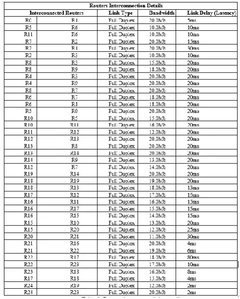
Table 3: Routers interconnectivity details
I.Simulating Links and nodes Failure
During the course of the simulation we simulated different links and nodes failure the details the link and nodes failure are mentioned in table 4 and 5 respectively.
Table 5: Showing nodes failure and restoration time
LinkFailure LinkRestoration
Time Nodes Time Nodes
10 R4 R9 15 R4 R9
16 R6 R1 22 R6 R1
47 R14 R9 52 R14 R9
73 R18 R13 75 R18 R13
85 R15 R20 89 R15 R20
Node/RouterFailure Node/RouterRestoration Time Routers Time Routers
25 4 30 4
40 12 43 12
55 17 59 17
70 20 75 20
5. Simulation Results
We used ns2 version 2.35 to perform the simulation. We used TCP protocol and FTP application to send packets towards the server, the course of the simulation was 100 seconds. We analyze the results on the basis of following four parameters.
1) Paket drop rate
2) Bandwidth / Link utilization 3) End to End delay
4) Throughput
Packet Drop Rate for Distance Vector, Link
State and Session Routing Protocol
The comparison graph for distance vector, link state and session routing protocols for packet drop rate in figure 2 shows that session routing protocol has highest packet drop rate as compared to distance vector and link state routing protocol. Distance vector routing protocol has least drop rate as compared to LS and session routing protocols.
Bandwidth Utilization for Distance Vector,
Link State and Session Routing Protocol.
Figure 3: Bandwidth Utilization for Distance Vector, Link State and Session Routing Protocol
Figure 3 shows bandwidth comparison of all three routing protocols, apart from distance vector routing protocol which has unusual bandwidth
gain, link state and session routing protocol bandwidth behavior is almost similar to each other.
End to End Delay Comparison for DV, LS
and Session Routing Protocols
Figure 4: End to End Delay Comparison for DV, LS and Session Routing Protocols
Figure 4 shows comparison graph for end to end delay all three routing protocols unlike distance vector routing protocol link state routing protocol end to end delay is much stable as compared to DV and Session routing protocols.
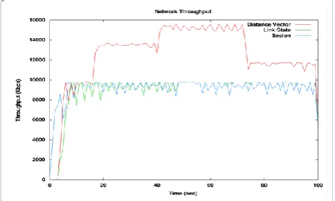
Throughput Utilization for Distance Vector,
Link State and Session Routing Protocol.
Figure 5 shows throughput comparison of all three routing protocols, apart from distance vector routing protocol which has unusual throughput gain, link state and session routing protocol throughput is almost similar during half of the simulation time later on Link state throughput become much more stable.
Figure 5: Throughput Utilization for Distance Vector, Link State and Session Routing Protocol.
6. Conclusion
We observe that distance vector routing protocol has better link utilization than Session and Link state routing protocol. Average Link utilization of distance vector routing protocol is better.
Session routing protocol has very high end to end delay as compared to distance vector and link state routing protocol.
Similarly, network throughput of distance vector routing protocol is better than link state and session routing protocol. We observed that Link state throughput was quite steady as compared to session routing protocols.
References
[1] Static Routing, https://en.wikipedia.org/wiki/Static_routing
[2] Internet Engineering Task Force (IETF), https://www.ietf.org/
[3] Houassi Hichem, Bilami Azeddine,” IP address lookup for Internet
routers using cache routing Table”, IJCSI, International Journal of
Computer Science Issues, Vol. 7, Issue 4, No 8, July 2010.
[4] Network Working Group, C. Hedrick Request for
Comments: 1058, Rutgers University June1988,
https://www.ietf.org/rfc/rfc1058.txt
[5] Network Working Group J. Moy Request for Comments: 2328 Ascend Communications,
Inc, April
1998,https://www.rfceditor.org/rfc/rfc2328.t xt
[6] Session Routing Protocol,
http://www.isi.edu/nsnam/ns/doc/node318.html
[7] Deepankar Medhi,Karthikeyan Ramasamy, Network Routing Algorithms, Protocols, and
Architectures, Morgan Kaufmann, San Francisco, (2007). [8] Donald B. Johnson, “A Note on Dijkstra's Shortest Path Algorithm”, Journal of the ACM (JACM),
Volume 20 Issue 3, July 1973 , Pages 385-388.
[9] Shubhi, Prashant Shukla, “Comparative Analysis of Distance Vector Routing & Link State
Protocols”, International Journal of Innovative Research in Computer and Communication