Stone's representation theorem

CSUSB ScholarWorks

CSUSB ScholarWorks

Theses Digitization Project John M. Pfau Library

2007

Stone's representation theorem

Stone's representation theorem

Ion Radu

Follow this and additional works at: https://scholarworks.lib.csusb.edu/etd-project

Part of the Mathematics Commons

Recommended Citation Recommended Citation

Radu, Ion, "Stone's representation theorem" (2007). Theses Digitization Project. 3087.

https://scholarworks.lib.csusb.edu/etd-project/3087

A Thesis

Presented to the

Faculty of

California State University,

San Bernardino

In Partial Fulfillment

of the Requirements for the Degree

Master of Arts

in

Mathematics

by

Ioan Radu

A Thesis

' Presented to the

Faculty of

California State University,

San Bernardino

by

Ioan Radu

March 2007

Approved by:

Dr. Belisario Ventura, Committee Member

___________

Date

II

Dr. Zahid Hasan , Committee Member

Dr. Peter Williams, Chair, Department of Mathematics

Jr. Joseph Chavez Graduate Coordir

Abstract

In mathematics, a representation theorem is a theorem th a t states th a t every

abstract structure with certain properties is isomorphic to a concrete structure. My

purpose in this thesis is to analyze some aspects of the theory of distributive lattices -

in particular the Representation Theorems:

• Birkhoff’s representation theorem for finite distributive lattices

• Stone’s representation theorem for infinite distributive lattices

The representation theorem of G arrett Birkhoff establishes a bijection between

finite posets and finite distributive lattices. Stone’s representation theorem for lattices

states th a t every distributive lattice is isomorphic to a sublattice of the power set lattice

of some set. As can be seen, each of these results gives a concrete realization for (abstract)

Acknowledgements

I would like to express my appreciation to my committee chair, Dr. Gary

Griffing, for this guidance, time, energy, and support in producing this thesis. I would

also like to thank the professors on my committee, Dr. Zahid Hasan and Dr. Belisario

Table of Contents

A b stract iii

A cknow ledgem ents iv

List o f Figures vii

1 Introd u ction 1

2 Ordered S ets 3

2.1 Ordered Sets ... 3

2.2 Chains and A n tic h ain s... 4

2.3 Order Isom orphism ... 4

2.4 P o w e rs e ts ... 4

2.5 The Covering R e la tio n ... 5

2.6 D ia g r a m s ... 5

2.7 The Dual of an Ordered S e t ... 6

2.8 Bottom and T o p ... 8

2.9 Maximal and Minimal E lem ents... 8

2.10 Sums and Products of Ordered Sets ... 9

2.11 Down-Sets and U p - S e t s ... 11

2.12 Maps Between Ordered S e t s ... 11

3 L attices and C om plete L attices 13 3.1 Lattices as Ordered S e t s ... '. . 13

3.2 Lattices as Algebraic S t r u c t u r e ... 17

3.3 Sublattices, Products and H om om orphism ... 19

3.4 Ideals and F il te r s ... 23

4 C om plete L attices and Q -structure 27

5 Join-irreducible E lem ents 31

7 R ep resen ta tio n Theorem : th e F in ite Case 45

8 R ep resen tation Theorem : th e G eneral Case 56

9 C onclusion 64

List of Figures

2.1 The Construction of Diagrams ... 6

2.2 Examples of D ia g ra m s ... 7

2.3 The Dual Ordered S e t ... 8

2.4 Maximal Elements and Maximum ... 9

2.5 Maps Between Ordered S e t s ... 12

3.1 Upper and Lower B o u n d s ... 14

3.2 Join and Meet ... 15

3.3 Sublattices ... 20

3.4 I d e a l s ... 24

5.1 Join-irreducible E l e m e n t s ... 32

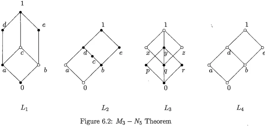
6.1 M3 — TVs L a ttic e s ... 40

6.2 M3 — T h e o r e m ... 40

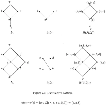
7.1 Distributive L a t t i c e s ... 49

7.2 Non-distributive L attices... '... 50

Chapter 1

Introduction

In Mathematics, representation theorems help us to investigate unknown ab­

stract structures, by allowing us to consider more well known concrete structure. At

the core of every representation theorem is a stucture preserving map from the abstract

structure to the concrete one. The original structure is studied via its image under this

map.

According to Johnstone [3] the birth of abstract algebra can be traced to a paper

of Cayley on group theory (1854). Universal algebra established itself in the 1930’s as a

unifying tool for the theory of groups, modules, rings and lattices.

The topologist M. Stone introduced in 1934 the notion of topology to algebra

and proved his famous representation theorem for finite Boolean algebras [6]. In his

work, Stone proved th at every finite Boolean algebra can be realized as the full power

set of the set of atoms of the Boolean algebra; each element of the Boolean algebra

bijectively corresponds to the set of atoms (minimal elements) below it (the join of which

is the element). This power, set representation can be constructed more generally for any

complete atomic Boolean algebra; however in these cases, the image of the representation

is not the full power set.

Independently at around the same time (1934), G arrett Birkhoff proved a rep­

resentation theorem for finite distributive lattices [7] (in this thesis see Theorem 7.4). It

states th a t every finite distributive lattice is isomorphic to a lattice of down-sets of the

poset of join-irreducible elements. This establishes a bijection between the class of all

In the same period of time (1936) Stone discovered a m ethod to extend his

representation result for finite Boolean algebras to arbitrary Boolean algebras [4], [6]

and Birkhoff adapted it to arbitrary distributive lattices [7] (see Theorem 8.6 in this

thesis).

In this work, we focused on distributive lattices and give a representation result

for both the finite and infinite cases. In each case, the result is due to both, Birkhoff

and Stone, and is purely algebraic in th a t no topology is used.

Throughout this thesis, unless otherwise stated, the references for definitions,

lemmas, corrollary, etc, can be found in Davey and Priestley [1] and Gratzer [2]. A nice

Chapter 2

Ordered Sets

We begin by introducing the notion of order. When we think about order we

refer to more th an one objects. An ordering is a binary relation on a set of objects that

compares them. Greater than, taller, less or equal, are examples of ordering.

2.1

O rdered S ets

D efinition 2.1. Let P be a set. A n o rd er (or p a rtia l order) on P is a binary relation

< on P such that, for all x , y , z G P,

(i) x < x Reflexivity,

(ii) x < y and y < x imply x = y Antisymetry,

(Hi) x < y and y < z imply x < z Transitivity.

A set P equipped with an order relation < is said to be an ordered set (or

partially ordered set). We’ll refer to the ordered set using the shorthand p o set and

we write (P; <) when it is necessary to specify the order relation. On any set P, the

discret order, and ‘< ‘ meaning strict inequality are order relations. We use x < y

and y > x interchangeably, and write x £ y to mean ‘r < y is false1. Also, we use x || y

when x is not comparable with y. We can construct new ordered sets from existing ones.

If P is an ordered set and Q a subset of P , then Q inherits an order relation from P;

given x ,y G Q, x < y in Q if and only if x < y in P . We say th at Q has the induced

2.2

C hains and A ntichains

D efin ition 2.2. Let P be an ordered set. Then P is a c h a in if, for all x ,y G P, either

x < y or y < x. A t the opposite extreme from a chain is an antichain. The ordered set

P is an a n tic h a in if x < y in P only if x = y.

The set R of all real numbers, with its usual order, forms a chain. The natural

numbers N, the integers Z, and the rational numbers Q, also have a natural order making

them chains.

We denote the set N U {0} = {0,1,2,3,...} by No- This set with the order in

which 0 < l < 2 < 3 < . . . becomes a chain. In particular, in the finite case we will use

the symbol n to mean the chain 0 < 1 < 2 < ... < n — 1.

The length of a finite chain C is |C| — 1. A poset P is said to be of length n,

where n is a natural number, iff there is a chain in P of length n and all chains in P

are of length < n. A poset P is of finite length if and only if it is of length n, for some

natural number n.

2.3

Order Isom orphism

We say that P and Q are (order-) isom orphic and write P = Q, if there

exists a map ip from P onto Q such th at x < y in P if and only if <p(x) < ip(y) in Q.

Then <p is called an order-isom orphism . This map is neccesarily one-to-one and onto.

2.4

Pow er sets

Let X be any set. The powerset P ( X ), consisting of all subsets of X , is ordered

by set inclusion: for A, B e -P(X), we define A < B if and only if A C B . Any subset of

P (A ) inherits the inclusion order.

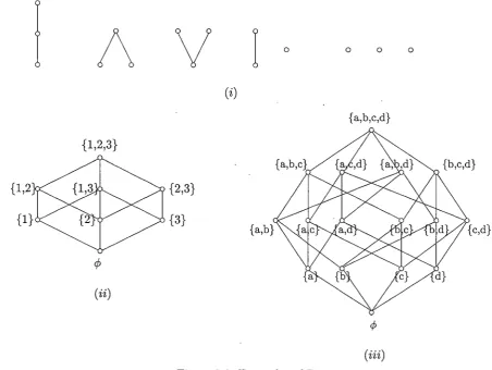
For example if we have set X consisting of 3 elements: X = {1,2,3} the powerset

P (X ) has the following elements shown in Fig. 2.2 (ii):

P (A ) = {</>, {1}, {2}, {3}, {1,2}, {1,3}, {2,3}, {1,2,3}}

2.5

T h e C overing R elation

Let P be an ordered set and let x ,y G P. We say x is covered by y (or y covers

re), and write x -< y or y >- x, if x < y and x < z < y implies z = x. The latter condition

is demanding th a t there be no element z of P with x < z < y. If P is finite, x < y if and

only if there exists a finite sequence of covering relations x — xo X\ x n = y.

For example:

• In the chain N, we have m -< n if and only if n — m + 1.

• In R, there is no covering relation since there are no pairs x .y such th a t x y.

• In P (X ), we have A B if and only if B = A U {6} for some b E X \ A .

2.6

D iagram s

Let P be a finite ordered set. We can represent P by a configuration of cir­

cles (representing the elements of P ) and interconnecting lines (indicating the covering

relation).

To construct a diagram for a power set, we need first to associate to each point

x E P, a point p(x) of the Euclidian plane R 2, depicted by a small circle with center

at p(x). Then for each covering pair x -< y in P , take a line segment l(x ,y ) joining the

circle at p[x) to the circle at p(y). We need to do this in such a way that:

(a) if x -< y, then p(x) is ‘lower' than p(y) (that is, in standard cartesian coordinates,

has a strictly smaller second coordinate).

(b) the circle at p(z) does not intersect the line segment l(x, y) if z x and z / y.

Figure 2.1 (i) shows two alternative diagrams for the ordered set P = {a, b, c, d}

in which a < c, b < c, a < d and b < d. We can see also th at a || b and c || d. In Figure

2.1 (ii) we have drawings which are not legitimate diagrams for P . In the first c is ‘lower'

than b, even in our set b < c, so the 3(a) rule in 2.6 is violated. In the second the line ad

intersects the circle c but c a and c / d, so the 3(b) rule is violated. In Figure 2.1(iii)

we have the following relations:

• c < e < g

• a||c, 6||c, d||e, f\\g, and so on.

We have defined diagrams only for finite ordered sets. It is not possible to rep­

resent the whole of an infinite ordered set by a diagram, but if its structure is sufficiently

regular, like in Figure 2.1(iv), we can sugest how the ordered set looks like. Figure 2.2

contains diagrams for a variety of ordered sets: ■

(i) all possible ordered sets with three elements.

(ii) the power set P{1,2,3}

(iii) the power set 7?{a,b,c,d}

2.7 T h e D u al o f an O rdered Set

For any ordered set P there exists a new ordered set P s (the dual of P ) defined

<t>

{Hi)

Figure 2.2: Examples of Diagrams

for the dual can be obtained simply by ‘turning upside down' the original diagram, as

we can see in Figure 2.3.

We can observe th a t for each statm ent about the ordered set P there coresponds

a statem ent about P s. For example, in Figure 2.3 we can say th at in P there exists a

unique element e covering exactly three others elements b, c, d, while in P 5 there exists a

unique element a covered by exactly three others elements b, c, d. In general, given any

statem ent $ about ordered sets, we obtain the dual sta tem en t <f>'5 by replacing each

occurrence of < by > and viceversa.

T he duality principle. Given a statement $ about ordered sets which is true

Figure 2.3: The Dual Ordered Set

2.8

B o tto m and Top

D efinition 2.3. Given an ordered set P , we say P has a b o tto m element if there exists

± G P with the property that ± < x for all x € P.

Using the duality principle, we get the definition of top element

D efinition 2.4. Given an ordered set P , we say P has a to p element if there exists

T G P with the property that T > x for all x G P.

L em m a 2.5. I f an ordered set P has bottom, then this is unique.

Proof. Let P be an ordered set, and let ± i and ±2 be two bottoms of the ordered set.

If l i G P is a bottom of P then ±1 < x for all x E P. T hat implies ±1 < ±2> since

± 2 £ P- If J-2 G P is a bottom of P then ±2 < x for all x e P, in particular, ±2 < -Li since ±1 is an element of P. Therefore ±1 = ±2 by the antisymmetry of <. □

As a consequence of the duality principle, if an ordered set P has top, then this

is unique. In C), we have ± = 4> and T = X . A finite chain allways has bottom

and top elements, but an infinite chain need not have. For example the chain (N; <) has

bottom element 1 and no top element, while (Z ;<}, the chain of integers has neither

top nor bottom.

2.9

M axim al and M inim al E lem ents

D efinition 2.6. Let P be an ordered set and let Q C P. Then a G Q is a m a x im a l

We denote the set of all maximal elements of Q by Max Q. If Q has a top

element, Tq, then Max Q = Tq and Tq is called the m axim um element of Q.

A minimal element and minimum are defined dualy. A minimum element of Q is

a maximum element of Qs and minimum of Q is maximum of Qs . The set of all minimal

elements of Q is denoted MinQ. If Q has a bottom element, ±q, then MinQ = Tq and Tq is called the m inim um element of Q.

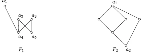
Figure 2.4: Maximal Elements and Maximum

In the Figure 2.4 P i has maximal elements 01,02,^3 and minimal elements 04

and <35 but no maximum or minimum. P2 has a± as maximum and a% as minimum.

2.10 Sum s and P ro d u cts o f Ordered S ets

Two ordered sets are join together in several different ways. In each of these

constructions we require th at sets being joined are disjoint.

D efinition 2.7. Let P and Q be disjoint ordered sets. The lin e a r s u m P ® Q is defined

by taking the following order relation o n P U Q : x < y if and only if

x ,y G P and x < y in P,

or x ,y G Q and x < y in Q,

or x G P and y G. Q.

A diagram for P © Q is obtained by placing a diagram for P directly below

a diagram of Q and adding a line segment from each maximal element of P to each

D efinition 2.8. Let P i,...,P n be ordered sets: The C a rte sia n p r o d u c t P i x ... x Pn is

an ordered set with the coordinatewise order defined by

(®i, ■■■, x n) < ( y i , y „ ) if and only if (V iX < y; in Pi

A product P x Q is drawn by replacing each point of a diagram of P by a

copy of a diagram of Q, and connecting corresponding points. In particular, 2” is the

cartesian product of the chain 2, n times.

L em m a 2.9. Let X — {1, 2, 3,..., n} and define p : P (X ) — > 2n by <^(A) = (e i,..., en)

where

1 (i £ A)

0 (i <£ A)

Then p is an order-isomorphism.

Proof. To show th at p is an isomorphism, we have to show :

(i) A < B implies p(A ) < p (B )

(ii) p is one-to-one

(iii) p is onto

Proof of (i)

Let A, B e P(X~) be two subsets of A, with A C B and let 99(A) = (e i,...,e n) and

p (B ) = (<5i,..., dn). We need to show th at p (A ) < p (B fi A C B <=> (Vi) i e A implies

i E B . This is equivalent to (Vi)ei = 1 implies = 1, which is equivalent to (Vi)e^ <

Si-This later statem ent gives us 99(A) < p(B } in 2n.

Proof of (ii)

Given p : P (A ) — > 2n , 99(A) = (ei,...,e„) and p (B ) = (5i,...,5„) and 99(A) = 99(B).

Then, since 99(A) = 99(B), we have (ei,C2, ...,en) = (5i, d%, ■■■, dn). This implies that

= (Vi) i = l,2 ,...n .

We can have either i £ A or i A. If i £ A, then Cj = 1, which implies di = 1.

Thus, i E B and A C B. If i A, then = 0 = di. Hence i B . Thus by contrapositive

B C A. Therefore p is one-to-one.

Proof of (iii)

2.11

D ow n -S ets and U p -S ets

D efinition 2.10. Let P be an ordered set and Q C P.

(i) Q is a d o w n -se t if, whenever x € Q, y G P and y < x, we have y e Q.

(ii) Dually, Q is an u p -s e t if, whenever x e Q, y G P and y > x, we have y G Q.

We can think about a down-set as one which is ‘closed under going down’ and

about an up-set as one which is ‘closed under going up’.

Given an arbitrary subset Q of P, we define:

‘down Q ’ : [ Q := {y E P \ (3x E Q) y < x}

‘down x ’ : J. x := {y E P | (y < a;)}

‘up Q’ : I Q - = { y e P | (3x G Q) y > x}

‘up x ’ : | x := {y E P | (y > a:)}

Up-sets (down-sets) of the form | x ( j x) are called principal.

The family of all down-sets of P is denoted by O (P ) and is itself an ordered

set, under the inclusion. When P is finite, every non-empty down-set Q of P is of the

form (Ji=i J- x > us the reader may easy verify.

E xam ple 2.11. In Figure 2.1(iii) the sets {c}, {a, b, c, d, e} and {a, b, d, f } are all

down-sets, but the set {b, d, e} is not a down set because a, b and a £ {b, d, e}. The set {e, f , g}

is an up-set, but {a, b, d, f } is not.

E xam ple 2.12. I f P is an antichain, then O {P )= P {P f

E xam ple 2.13. I f P is the chain n, then O (P) consists of all the sets J. x fo r x E P,

together with the empty set.

E xam ple 2.14. I f P is the chain Q of rational numbers, then O (P ) contains the empty

set, Q itself and all sets j x (for x E Q / We have also other sets in 0 ( P ) , like j aj\{a:}

(for x E<Q>) and {y E Q \y < a} (for a E R \ Q /

2.12

M aps B etw een O rdered S ets

(i) o rd er-p rese rv in g if x < y in P implies < p(y) in Q;

(ii) an ord er-em b ed d in g (and we write p : P Q) if x < y in P if and only if

<p(x) < <p(y) in Q;

(Hi) an o r d e r -is o m o rp h is m if it is an order-embedding which maps P onto Q

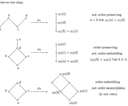
In Figure 2.5 ip± is not order-preserving, since a < v b u t,^ i(o ) > <pi(b). On the

other hand <p2 is order-preserving but is not order-embedding. Note th a t p>2(b) < <p2(c)

but b / c. The function </?3 is order-embedding but not order-isomorphism, since is not

one-to-one map.

¥>2

9 ^ ( e )

9 <^2(c) = <P2(d)

° (^2(a) = <fi2(b)

not order-preserving

a < b but p i (a) > <pi (b)

order-preserving

not order-embedding

(<P2(b) < ip2(c) but b ft c)

Figure 2.5: Maps Between Ordered Sets

order-embedding

not order-isomorphism

Chapter 3

Lattices and Complete Lattices

Two of the most im portant classes of ordered sets are lattices and complete

lattices. In this chapter we present the basic theory of such ordered sets.

3.1

L attices as O rdered S ets

D efinition 3.1. Let P be an ordered set and let S Q P . A n element x E P is an

u p p er-b o u n d of S if s < x for all s E S . Dually an element x E P is an low er-bound

of S if s > x for all s E S.

The set of all upper-bounds of S is denoted by S u and the set of all lower

bounds by S 1-.

S u {x E P|(Vs E S') s < x} and S l := {x E P|(Vs E S') s > x}.

Since < is transitive, S w is an up-set and S l is a down-set. If S u has a least element x.

then x is called the least upper bound of S. The least upper bound of S is also called

the suprem um of S and is denoted by sup S. If S l has a greates element x, then x is

called the greatest lower bound of S. The greatest lower bound of S is also called the

inflm um of S and is denoted by inf S'. The supremum of S exists if and only if there

exists x E P such that

(Vy E P )[(fys E S ) s < y ) O x < y]

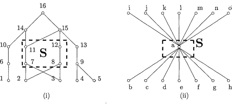
In ordered set (i) from Figure 3.1 S — {7,8,11,12}. The elements 15, 16 are the only

of all upper bounds and 15 is the sup S', since 15 is the least element of {15,16}. The

set S l = {2,3} is the set of all lower bounds and we have no infimum.

Figure 3.1: Upper and Lower Bounds

In ordered set (ii), S = {a}, S u = { i,j,k,l,m,n,o} , S l = { a,b,c,d,e,f,g,h}. Here

we do not have any supremum or infimum.

R em ark 3.2. There are two extreme cases for S as subset of P: when S is empty or S

is P itself. I f S is the empty s e t , then every element x 6 P satisfies s < x for all s 6 S.

Thus (f>u = P and hence sup <f> exists if and only if P has a bottom element, in which

case sup f> = ± . Dually, in f <j> = T whenever P has a top element.

N otation . We write a: V y (read as ‘x join y’) in place of sup {x, y} when it

exists and x A y (read as lx m eet y’) in place of inf {a;,y} when it exists. From this

observe th a t the commutative law holds. T hat is, x V y = y V x and similarly for meet.

Similary we write \Z S (the join o f S) and f \ S (the m eet o f S') instead of sup S' and

inf S' when these exist.

R em arks 3.3.

(1) Let P be an ordered set. I f x , y & P and x < y , then {a;, y }u = } y and {», y } 1 = | x.

x V y — y and x f \ y = x whenever x < y. In particular, since < is reflexive, we

have x V x = x and x / \ x = x.

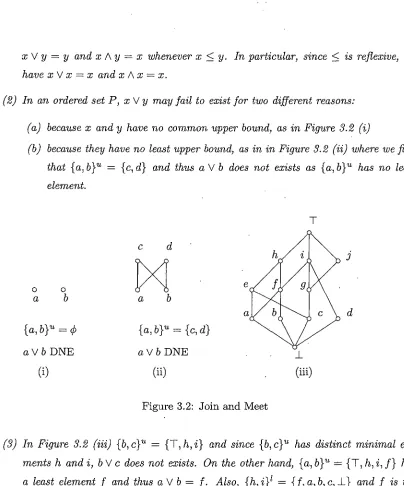
(2) In an ordered set P, x \ / y may fail to exist for two different reasons:

(a) because x and y have no common upper bound, as in Figure 3.2 (i)

(b) because they have no least upper bound, as in in Figure 3.2 (ii) where we find

that {a, b}u = {c, d} and thus a V b does not exists as {a, b}u has no least

element.

o o

a b

{a, b}u = fi

a \/ b DNE

(i)

Figure 3.2: Join and Meet

(3) In Figure 3.2 (Hi) {b, c}“ = { T ,/i,i} and since {6, c}u has distinct minimal ele­

ments h and i, b \/ c does not exists. On the other hand, {a, b}u = {T, h ,i, f } has

a least element f and thus a V b = f . Also, {h, i} 1 = { f, a, b, c, ± } and f is the

greatest element, therefore h A i = f .

D efinition 3.4. Let P be a non-empty ordered set.

(i) I f x V y and x f \ y exist for all x ,y € P , then P is called a la ttice

(ii) I f \ / S and f \ S exist for all S C P , then P is called a co m p lete la ttice

E xam ple 3.5. Each of K, Q, Z, and N is a lattice under its usual order. By Re­

mark 3.2(1), if x < y then a; V y = y and x A y = x. Hence, every chain is a lattice in

E xam ple 3.6. None of the lattices R, (Q>,. Z, and N is complete; every one lacks a top

element, and a complete lattice must have top and bottom.

E xam ple 3.7. For any set X , the ordered set {P (X f, Q)is a complete lattice in which

\ / { A i | z e i } = (J{A ; \ i e I} ,

f \ { A i | i G 1} = P ){ A \ i S I} .

Proof. First, we note th at we shall indicate the index set by subscripting it. Thus,

instead of (J { A | » 6 f} we write (Jigj A i, and instead of H { A | i € 1} we write Qigl Ai.

Let be a family of elements of P (X ). Since (Jig/ A D A j for all j E I, it follows th a t (Jigl Ai is an upper bound for {.AJieJ- Now, let B E P (X ) be another upper bound

of {>li}iej. Then B 3 Ai for a lii e I and hence B 3 (Jigj Ai. Thus (Jig/ A is indeed the

lowest upperbound of { A } is/ in P (X ). The assertion about meets is proved dually. □

E xam ple 3.8. With F/q = { 0 ,1 ,2 ,3 ,...} , a < b if and only if a|h, o V b = lcd(a, 6) and a / \ b = gcd(a, b) , (Ao; led; ged) is a lattice.

Proof. We’ll first prove th at the relation a < b iff a\b is an order relation. Since every

x E No is divisible by itself the relation is reflexive. If x, y E No, x\y and y\x imply x — y

and thus the relation is antisymmetric. Now, let x ,y , z E No, x\y and y\z. Then, there

exist p, q E No such th at y — x-p and z — y-q. T hat implies z = y • q = (x-p)-q = x-(p-q)

and x\z. Thus the relation is transitive. Therefore (No;lcd;gcd) is an ordered set.

Second we have to prove th at the lcm(a, b) and the gcd(a, b) are precisely a V b and a A b,

respectively. Let lcm(a, b) = c. T hat implies a\c and 6|c and by the definition of relation

in our ordered set, a < c and b < c. Since by definition c divides any other multiple

of a and b, c is the sup(a, b) and therefore lcm(a, b) = a V b. Dually we can show th at

gcd(a, 6) = a A 6. Therefore (No; led; ged) is a lattice. □ L em m a 3.9. Let P be a lattice. Then for all a, b,c,d E P,

(i) a < b implies a \/ c < bV c and a A c < b A c

Proof. For the (i) part let P be a lattice and a, b, c, d £ P and let a < b. Then by

Remark (1) above aVb = b. Consider the element b \/c = (a V b )V c (since aV& = 6). By

the associative and commutative laws (see next theorem) b Vc = (a V6) Vc = 6 V (aVc).

Using the definition of join, 6 V c > b and 6 V c > a V c. Therefore we have the result

a V c < b V c and the proof is complete. For the second part by Remark (1) above

a /\b = a. Consider the element a f \ c = (a A 6) Ac (since a A b = a). By associativity

a / \ c = a / \ ( b / \ c ) and by the definition of meet a A c < b A c.

For the (ii) part a < b implies a V b = b, and c < d implies c V d — d. Then

the element b V d in lattice P is equal to (a V b) V (c V d) and using the associative and

commutative laws is equal to (oV c) V (6 V d). Thus we have 6 V d — (a V c) V (6 V d) and

therefore, a V c < b V d. The element a A c in lattice P is equal to (a A b) A (c A d) since

aAc = a and cAd = c. Using the associative and commutative laws a/\c — (bf\d)/\(af\c).

Thus we have a A c < b A d. □

3.2

L attices as A lgebraic S tructure

Given a lattice L, we define binary operations join and m eet on the non-empty

set L by

a V b := sup{a, b} and a A b := inf {a, b} (a,b £ L)

In this section we view a lattice as an algebraic structure (L; V, A).

L em m a 3.10. C onnecting Lem ma.

Let L be a lattice and let a,b € L. Then the following are equivalent:

(i) a < b;

(ii) a V b = b;

(Hi) a /\b = a.

Proof We already showed in Remark (1) above that, (i) implies (ii) and (i) implies (Hi).

Now, assume (ii) a V b = b. We know from the definition of join th a t a < a ' i b. Thus,

a < a V b = b implies a < b which is (i). To show that (Hi) implies (i), we take a /\b = a

T heorem 3.11. Let L be a lattice. Then V and A satisfy, fo r all a ,b ,c E L,

(L I) (a V b) V c = a V (b V c)

(L2) a \ / b — b\l a

(L3) a V a = a

(L4) a \f (a Ab) = a

and

and

and (L3)5 a /\a = a

and (L4)5 a A (o V b ) =

(L \)5 (o Ab) A c = a A (b A c)

(L2)5 a A b = b /\ a

(associative laws)

(commutative laws)

(idempotency laws)

(absorption laws)

Proof. Let a,b G P and a < b. Then, {a, b}u = b | and {a, b}1 = a j, since the least

element of b | is b and the greatest element of a $ is a. Thus, a V b — b and a A b = a

whenever a < b. In particular if in the set {a, b} we let b = a, we get a V a = a and

a A a — a, which proofs L(4).

To prove L(2) we remember th at a V b = sup{a, b} and th a t is equal to

sup{b, o} = b V a.

To prove L(3) we’ll use the above lemma. If we have two elements belong to

the lattice L, both elements are less or equal to their join. In particular if our elements

are a and a A b, then a < a V (a A b). By Lemma 3.4 a /\ a V (a A b) = a and since a V a = a

(by L(3)), we have a V (a A b) = a.

To prove L (l) let a, b, c G L and d G {o, b, c}u be any upper bound of the

set {a, b, c}. If d is an upper bound of {a, b, c} then, by definition, d > a, d > b and

d > c, and moreover the upper bound d is an upper bound for any subset of {a, b, c}.

Thus, we have d G {a, b}u and d > c, which implies d > a V b and d > c, which implies

d G {a V b, c}“ . In the same time we can say th at d G {b, c}“ and d > a, which implies

d G {b V c, and thus d G {b V c, o}“ . Thus the set of {b V c, a}u = {bV c, a )u. That

implies th a t the two sets have the same least element and therefore (aVb)Vc = aV(bVc).

Note th a t the dual statements L (l)'5 — L(4)s are obtained simply by interchang­

ing the V and A. □

T heorem 3.12. Let (L-,\/,/\) be a non-empty set equiped with two binary operations

which satisfy (LI) — (L4) and (L I)5 — (L4)5 from 3.11.

(i) For all a,b G L, we have oV b = b if and only if a /\b = a

(Hi) With < as in (ii), (£; <) is a lattice in which the original operations agree with the

induced operations, that is, for all a,b € L,

a, V 6 = sup{a, 6} and a A b = inf {a, 6}.

Proof. Assume a V 6 = 6. From (£4)s we have a = a A (a V b) and replacing a V b by b,

we have a — a A.b. Conversely, assume a A 6 = a. Replacing in ?? (£4), (b A a) by a, we

get b = b\/ a. Thus the proof of (i) is complete.

Now define < as in (ii). By £3, a V a = a and since by assumption a < b if

a V b = b we have a < a which shows reflexivity. To verify antisymmetry suppose first

th a t a < b. T hat implies a V 6 = 6. Second, suppose b < a, which implies 6 V a = a.

Since by £2, a V b = b V a w e have a — b. To show th a t < is transitive let a,b ,c S £,

a < b and b < c. If a < b, then a V b = b and if b < c, then bV c — c. Replacing these two

joins in £1, a V (6 V c) = (aV b) V c we find th at a V c = b V c and since b V c = c we have

a V c = c which implies th at a < c. Thus < is reflexive, antisymmetric and transitive,

therefore is an order relation. (

W ith < and V defined as in (ii), to show th at a V b — sup{a, b} in the ordered

set (£; <) we need to show th at aVfc € {a, b}u and th at d E {a, b}u implies d > aVb. The

following equality (a V b) V a — (a V a) V b holds by the associativity and commutativity

laws of V. Since a V a = a, by ?? (£3), we have a V (a V b) = a V b. Using Lemma ??,

a V b > a. On the other hand (a V b) V b = a V (b V b) = a V b, which by (ii) implies

th a t o V b > b. These two results, a V b > a and a V b > b allow us to conclude that

o V b E {a, b}u. Now let d E {a, &}“ . We need to prove th at d > a Vf>. If d is an element

of the set of upper bounds of the set {a, b}, then d > a and d > b, which imply that

d V a = d and d V b — d. Looking at the element d V (a V b) we see th a t by associativity

this is equal to (d Va) \/b which equals d\/b, which equals d. Thus we have dV (a'ib) = d

and therefore, by (ii), d > a V b. □

3.3 S u b lattices, P ro d u cts and H om om orph ism

D efinition 3.13. Let L be a lattice and (j> ^ M E L . Then M is a su b la ttic e of L if

E xam ple 3.14. Any one element subset of a lattice is a sublattice. More generally a

non-empty chain in a lattice is a sublattice.

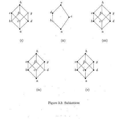
E xam ple 3.15. In the diagrams in Figure I I the shaded elements in lattice (?) and (??)

form sublattices. In {Hi}, since M = {b, e, g, d}, e,g e M but e V g — h and h M , the shaded elements do not form a sublattice. The shaded elements in {iv} do not form a

sublaitice, since e f\g = c and c is not shaded. In Figure I I {v} the shaded elements also do not form a sublattice since b y d = f and f is not in the subset of shaded elements.

E xam ple 3.16. The reader can easilly check that in Figure I I (w) the subset of shaded

elements forms a lattice in its own, without being a sublattice of L.

D efin ition 3.17. Let L and K be lattices with the ordered set L x K . We define V and

A coordinatewise on L x K , as follows:

G l, fel) V (Z2, fo ) = G l V Z2, ki V fo ) G l, fci) A (Z2, ^2) = G l A ^2, k t A kf)

It is routine to check th a t L x K satisfies the identities ?? (LI — (L4)5 and therefore is a lattice.

D efinition 3.18. Let L and K be lattices. A map f : L —> K is said to be a h o m o ­

m o r p h is m if f is jo in -p re se r v in g and m eet-p reservin g , that is, for all a,b G L,

f ( a V &) = / ( a ) V f(b) and f( a Ab) = f(a ) A f(b).

A bijective homomorphism is an isom orphism . If f : L —> K is a one-to-one

homomorphism, then /(L ) is a sublattice of K isomorphic to L and we refer to f as an

em bedd ing map.

E xam ples 3.19. In Figure 2.5, recall that <pi is not order-preserving since a||c and ip(a) > <p(c) but each of tp2,(p3,y>4 is an order preserving map. The map ip2 is an

homomorphism, the remainder are not. The map preserves joins but does not preserve

all meets. The map 723 is meet preserving but does not preserve all joins.

P ro p o sitio n 3.20. Let L and K be lattices and f : L —> K a map.

(i) The following are equivalent:

(a) f is order-preserving;

(b) (Va, b e L ) f ( a V b) > / ( a ) V f(b); (c) (Va, b E L ) f( a Ab) < f(a ) A f(b);

(ii) f is a lattice isomorphism if and only if it is an order-isomorphism.

Proof.

P art G) fa implies b).

(by Lemma ??),

(since the map / is order preserving)

(by Lemma ??).

(ya , b e L ) f (a \/b) > f (a) V f (fy.

Given a,b E L and a < b we have:

a V b = b

which implies / ( a V b) = f(b)

and /(a ) < f(b)

which implies /( a ) V f(b~) — f(b)

Using (L3) from Theorem 3.5, bVb — b. T hat implies /(b) V f(b) — f(b ). Replacing here

the values for f(b] found above, we have:

(/(« ) V f(by) V / ( a V b) = f ( a V b)

and therefore, by Lemma ??,

f ( a Vb) > f(a ) V f(b).

P art (2) (b implies a).

Given (Vo, b E L), a < b and / ( a V b) > f(a ) V /(b), we need to show th a t / ( a ) < f(b).

Given a,b E L and a < b we have a V b = b. Replacing this in / ( o V b) > /(o ) V f(b) and

using the fact /(a ) V f(b) > / ( a ) we obtain

f(b) > f(a ) V /(b ) > /(a )

and therefore / ( a ) < f(b~) what we needed to show.

P art (i) (o implies c). Let L and K be lattices and f : L K an order-preserving map,

we need to prove th at (Vo, b E L)

Given a.b E L and a < b we have:

a A b = a

which implies /( o A b) = /(a )

and /( a ) < /(b)

which implies /( a ) A /.(b) = /( a ) (by Lemma ??).

Using (L3)5 from Theorem 3.5, a A a = a. T hat implies /(o ) A /(o ) = f(a ). Replacing

here the values for /(a ) found above, we have:

(/(a ) A /(b)) A / ( a A b) = / ( a A b)

and therefore, by Lemma ??,

f ( a V b) > /(o ) V /(b).

(by Lemma ??),

(since the map / is order preserving)

P art (i) (c implies, a).

Given (Va, b G L), a < b and f ( a A £>) < f(a ) A f(b), we need to show th a t f(a ) < f(b).

Given a,b & L and a < b we have a A b = a. Replacing this in f ( a A b) < f(a ) A f(b) and

using the fact f(a ) A f(b ) < f(ti) we obtain

/(o ) < /( a ) A /(b ) < f(b)

and therefore f(a ) < f(b') what we needed to show.

P art (n) (=>)

Given f one -to-one, a, b elements of lattice with a < b and f ( a V b) — f( a ) V f(b) we need to show th at f(a ) < ffb ). In the given = /( a ) V ftff) replace a V b by b,

an d o b ta in

/(&) = /( a ) V /(b),

which implies f(a ) < f(b) (by Lemma ??).

P art (ii) (<s=) Given a,b G L, a < b implies /( a ) < f(b), we need to show th at f is bijective and preserves join and meet. Since f is order isomorphism, f is one-to-one and

onto (see 2.3). Since f is surjective there exists c G L such th at /( a ) V f(b ) = f(c ). By Lemma ?? /(a ) < /(c ) and f(b) < f(c ). Since f is order embedding, a < c and b < c.

Hence a V b < c. Since f is order isomorphism, /(a ) V b) < /(c ) = / (a) V /(b ) and thus

/ ( a ) V b) < / ( a ) V f ( b f By (i), f ( a V b > f(a ) V f(b ). Thus f ( a V b) = / ( a ) V /(b) and therefore preserves join. To show th a t / preserves meet it is enough to change

join with meet and < with >. Therefore, since / is surjective there exists c G L such th a t /( a ) A /(b) = f(c ). By Lemma ?? /(a ) > /(c ) and /(b ) > /(c ). Since / is

order embedding, a > c and b > c. Hence a A b > c. Since / is order isomorphism,

/(aA b) > /(c ) = /(a )A /(b ) and thus /(aA b) > /(a )A /(b ). By (i), /(aA b) < /(o )A /(b ).

Thus f ( a A b) = f ( a ) V and therefore preserves meet. Since / preserves join and

meet, / is a lattice isomorphism. □

3.4 Ideals and F ilters

D efinition 3.21. Let L be a lattice. A non-empty subset J of L is called ideal if

(ii) a 6 L, b G J and a < b imply a € J.

More compactly we can say th at an ideal is a non-empty down set closed under

join.

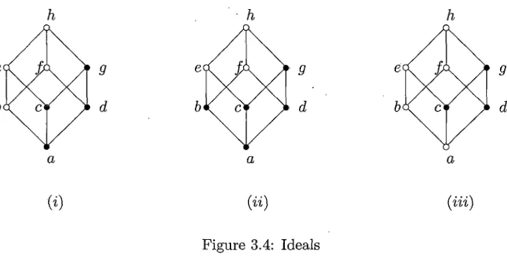
In Figure 3.4 the shaded elements in (i) form an ideal. The shaded elements

in {ii} do not form an ideal, since b, c G J but b V c J. In the same way, the shaded

elements in {in} do not form an ideal, since a G L, b e J and a < b, but a & J (the set

of shaded elements is not a down-set).

9

d

9

d

{i} {ii} {Hi}

Figure 3.4: Ideals

A dual ideal is called a filter. T hat means a filter is defined as a non-empty

subset G of L, such that:

(i) a, b € G implies a A b E G,

(ii) a E L, b G G and a > b imply a G G.

The set of all ideals (filters) of L is denoted by 1{L} {LF{L}}, and carries the

usual inclusion order.

An ideal or filter is called proper if it does not coincide with L.

For each a E L. the set J. a is an ideal and | a is a filter. J. a is known as

principal ideal generated by a and f a as principal filter generated by a.

P ro p o sitio n 3.22. Let L be a lattice and J C L a non-empty subset. J is an ideal of

(1 ) a,b € J implies a V b G J,

(2) a e L, b G J implies a Kb E J

Proof. Let L be a lattice and J C L a non-empty subset. We need to prove th a t J C L

satisfies (i) and (ii) from Definition 3.22 if and only if it satisfies (1) and (2).

Proof of (=>). Given a,b G J and (1) and (2), we have to show th a t a A b G J. From the

given a < b and using Lemma ??, we have a Kb = a and since a G J, a A b G J.

Proof of (<=). Given a G L, b G J, a < b and (1) and (2), we have to show th a t a G J.

From the given a < b and using Lemma ??, we have a K b = a and since a K b G J,

a E J. □

P ro p o sitio n 3.23. Let L and K be bounded lattices and f : L K a {0,1} homomor­

phism. Then f - f i f f ) is an ideal and / _1(1) is a filter in L.

Proof. Given L and K bounded lattices and f : L —> K a {0,1} homomorphism prove

th a t / ~ 1(0) is an ideal. Then / _1(0) = {x E L \f(x ) = 0}. Let a,b G / _1(0). Now

a V b G L, since L is a lattice and / ( a V b) = /( a ) V f(b) since f is a homomorphism.

But /( a ) V /(&) = 0 V 0 = 0, since a,b G / _1(0). Thus a V b G / _1(0). Now let a G L,

b G / _1(0), and a <b. We need to show th a t a E / -1 (0).

a < b => a \/ b = b

=>- f( a V 6) = f(b)

=>/( a ) V /(&) = /(&)

=> f(a ) < f(b~) = 0

=> /( a ) = 0

= > a G / _1(0)

(by Lemma ??)

(since f is homomorphism)

(by Lemma ?? and since b E / _1(0))

(since L is a bounded lattice)

(since f is 0,1 homomorphism)

Therefore, / _1(0) is an ideal.

Given L and K bounded lattices and f : L —> K a {0,1} homomorphism prove

th a t / _1(1) is a filter. Let / _1(1) —> Il the image of 1. Then / _ 1 (1) = {a; G L \f( x ) = 1}. Let a, b E / _1(1). Now a Kb E L, since L is a lattice and f(a K b ) = f(a ) K f(fi) since f is

Now let a € L, b G f 1(1), and a > b. We need to show th at a G f 1(1).

a > b => a Ab = b

^ f ( a A b ) = f(b)

=> f(a ) A f(b)

= > /( a )A /( 6 ) = l

=> /(« ) = 1

^ a e f V l )

(by Lemma ??)

(since f is homomorphism)

(by Lemma ?? and since b G / _1(0))

(since L is a bounded lattice)

(since f is 0,1 homomorphism)

Therefore, / _1(1) is a filter. □

P ro p o sitio n 3.24. For any set X the following are ideals in P (X )

(a) all subsets not containing a fixed element of X ;

(b) all finite subsets.

Proof. Let X be a set and let xo G X .

Proof of (a). Let G be the set of all subsets of X not containing a fixed element xo G X .

Then

G = {A G P ( X ) | so i A}

Let A, B G G. If rco A and a;o B , then xq 0 A U B . Thus A U B E G. Now, let

A € G, B G PfiX) and B C A. If xq A and B C A we have xo $ B and thus B is an element of G. Therefore by definition, G is an ideal.

Proof of (b). Let G be the set of all finite subsets of X . Then

G = {A e PfiX) | A is finite}

Let A, B G G be finite sets. Since the union of two finite sets is a finite set, A U B G G.

Now let A E G, B E P ( X ) and B C A. Since B is a subset of a finite set is itself finite

Chapter 4

Complete Lattices and

Q-structure

Recall from Definition 3.4 th at a complete lattice is a non-empty set P such

th a t the join (supremum), \J S, and the meet (infimum), / \ S , exist for all subsets S of

P. First we list some immediate consequences of the definitions of least upper bound

and greates lower bound.

P ro p o sitio n 4.1. Let P be an ordered set, let S ,T C P and assume that \ / S, \ f T , f \ S

and / \ T exist in P.

(i) s < \ f S and s > f \ S for all s G S.

(ii) Let x G P ; then x < f \ S if and only if x < s for all s & S.

(Hi) Let x G P ; then x > \ f S if and only if x > s for all s G S.

(iv) \Z S < f \ T if and only if s < t for all t e T .

(v) I f S C T , t h e n \ f S < \ / T a n d f \ S > f \ T .

L em m a 4.2. Let P be a lattice, let S ,T C P and assume that \ / S, \J T , / \ S and / \ T

exist in P . Then

Proof. Since both supfS1) and sup(T) exist, to show th at the equality holds, it just needs

to be shown th a t the right side, sup(S') V sup(T), satisfies the definition for least upper

bound of the set S U T .

Upper bound: If x is in 5 U T , then x G S of x E T . Thus, x < sup(S') Vsup(T’).

Hence sup(S') V sup(T) is an upper bound of S U T.

Least upper bound: If y is an upper bound for S U T , then for each z in

S U T , z < y. This implies in particular th at y is an upper bound for S and an upper

bound for T. Thus, sup(S') < y and sup(T) < y. Therefore, sup (S’) V sup(T) < y and

sup(S') V sup(T) is the least upper bound for S U T. Therefore by definition of join

V (S 'U T ) = (\/ S') V

(V

the proof is complete. □

L em m a 4.3. Let P be a lattice. Then \ / F and / \ F exist fo r every finite, non-empty

subset F of P.

Proof. Let F C P, non-empty, consisting of n elements F — {a-x, 0,2, <23, •.. an}. Then

V F can be defined in the following way: define an element S'{oi,. . . , an} recursively by

S ^ aq ,. . . , an} = sup{ai, S{a2, ■ ■ ■, an } with n > 2 and S'{a} = a. For example for n = 4,

5 { o i , . . . , o n} = sup{ai,sup{a2,sup{a3,a4}}}. First we need to prove S { a i , . . . ,a n} is

an upper bound for the set { a i,. . . , an}. To show S {<21,..., an} > ai, Vi, 1 < i < n,

either aj_ = S'{ai} > or by induction on n S{a2, • • •, an} > ai. Second we need to prove

th at S' { a i ,. . . ,a n} is the least upper bound. Suppose b > ai, \/i. Then, by induction

on n, b > sup{a„_i, a„} = S'{a„_i, an}- If b > sup{ak,S { a k+i , . .., o„} = S { a k, . . . , an },

we have b > sup{afc_i, S {a k, . . . , a,n} = S {a k~T, ■ • ■, an}- Thus b > S '{ ai,. . . , an} and

therefore S {a ± ,. . . , an}

= V{°1,

From the last lemma and the discusion about top and bottom in Section 3.1

the following holds.

C orollary 4.4. Every finite lattice is complete

By examining the proof of Exemple 3.7 the following holds.

C orollary 4.5. Let C be a family of subsets of a set X and let be a subset of £.

-(™) V D ie/ Ai G £ , then N c{A i\i G 1} exists and equals f) i e / Ai.

Consequently, any (complete) lattice of sets is a (complete) lattice with joins and meets

given by union and intersection.

L em m a 4.6. Let P be an ordered set such that f \ S exists in P fo r every non-empty

subset S of P . Then V S exists in P for every subset S of P which has an upper bound

in P ; indeed, \J S — f \ S u .

Proof. Let S C P , with S Assume S has an upper bound in P. Therefore S u <f>.

By hypothesis, / \ S U G P. Let a = / \ S U. We must show th a t f \ S = a. By definition,

/ \ S is the least upper bound for S. Will now show th at a = / \ S u is also a least upper

bound for S. If s G S, we want s < a. But Vt G S u, s < t Thus s < f \ S u and a

is an upper bound. Now if b E .P is also an upper bound for S we have b G S u and

thus / \ S U < b. This implies f \ S u < b and a is the least upper bound for S. Therefore

f \ S u = \J S . □

T heorem 4.7. Let P be a non-empty orederd set. Then the following are equivalent:

(i) P is a complete lattice;

(H) N S exists in P for every subset S of P;

(Hi) P has a top element, T , and / \ S exists in P for every non-empty subset S of P.

Proof. Let S be a subset of complete lattice P. Since by Definition of complete lattice,

N S exist for every subset of P, (i) implies (ii) automatically. Also, it is easy to prove

th at (ii) implies (Hi). Since f \ S exists in P for every subset S of P, N S exists for empty

subset of P. Thus, by Remark 3.2, P has a top element and since by (ii), N S exists in

P for every subset S of P, obvious it exists for every non-empty subset S of P. Now,

by Lemma 4.6 V S exists in P for every subset S of P. Given by (Hi) th a t / \ S exists in

P for every subset S of P, we have th at P is a complete lattice, by definition. Thus we

just proved th at (Hi) implies (i), and the proof of the theorem is complete. □

This theorem has a simple corollary.

C orollary 4.8. L e tX be a set and let £ be a family of subsets of X ordered by inclusion,

(a) A ig /A £ £ f or every non-empty family {A }ig/ £ , and

(b) X E C .

Then £ is a complete lattice in which

/ \ A i = ^ ] A i,

\ / A i = ^ \ { B E C \ \ j A i Q B } .

ieJ iei

Proof. (£\ C) is a complete lattice if \J S and / \ S exist for all S € £■ Thus by theorem

4.7 it suffices to show th at £ has a top element and the meet of all subsets of £ exist

in £ . Since £ is a family of subsets of X , X is the top element of £ . Now, let {A i}je/

be a non-empty subset of £ . Then A ^g /A e £ , by given (a). By Corollary 4.5, / \ igl A

exists and is equal to Aig/ A - Therefore, since £ has a top element and / \ ieI A l exists,

by Theorem 4.7, £ is a complete lattice. Now

V A = / \ { A i \ i e I } u (since X is an upper bound of {A } and Lemma 4.6)

ieJ

= Q { £ e £|(Vi e 7) Ai C B }

= Q { £ e £ | l j A c £ }

is/

Chapter 5

Join-irreducible Elements

D efinition 5.1. Let L be a lattice. A n element L is jo in -irre d u c ib le if

(i) x 0 (in case L has zero or bottom Jl),

(ii) x = a V b implies x = a or x — b for all a,b G L,

Condition (ii) is equivalent to

(ii4) a < x and b < x imply a V b < x for all a, b G L.

A m eet-irreducible element is defined dually. We denote the set of all join-irreducible

elements of L by J ( L ) and the set of all meet-ireducible elements by M (L ).

E xam ple 5.2. In a chain, every non-zero element is join-irreducible. Thus if L is an

n-element chain, then J ( L ) is an (n — 1)-element chain.

E xam ple 5.3. In a finite lattice L, an element is join-irreducible if and only if has

exactly one lower cover (see Section 2.5). This makes J ( L ) extremely easy to identify

from a diagram of L. In Figure 5.1 the shaded elements are all join-irreducible.

E xercise 5.4. Consider the lattice (No; lcm-,gcd) defined in Example 3.8. A non-zero

element m G No is join-irreducible if and only if m is of the form pr , where p is a prime

and r G N.

Proof. Let

a

(i)

Figure 5.1: Join-irreducible Elements

Define a V b — lcm(a, b), a f\b = gcd(a, b) and a < b if and only if a\b.

(=> ) Given m £ No, m = p iei - p ^ 2 ---- Pkek, distinct primes, a join-irreducible element

of L. we need to prove th a t m is of the form pr. First we’ll prove th a t the powers e1

with 0 < i < k can not be all zeros. For th at, we need to show th a t 1 is the bottom of

the lattice L and thus is not join-irreducible. Let ± be the bottom of lattice L. That

implies ± < x for all x £ L, or ± |s . Thus, x — y • _L for some y E No- Now, since x can

be any element of L let x = 2. T hat implies the only acceptable values for ± are ± = 1

or ± = 2, since ± |x . If we let x = 3 the only acceptable values for ± are ± = 1 or ± = 3.

Since ± |x for every x E L, the ± must be 1. Therefore, since m is join-irreducible in L.

m can not be the bottom and the powers e1 with 0 < i < k can not be all zeros.

Suppose one of e^’s is not zero. Choose i with e,; > 0 and ej = 0, Vj i. Then

m = p f is of the form pr . Now, let m — p f ■ p f ■ ■ ■ -P^ wEh distinct p ’s and write

m = p f1 • k, where k = p f ■ ... p ^ , ej > 0, j E { 2 ,..., n}. If k / 1, lcm (pf1 • k = m and

by hypothesis m is join-irreducible. This implies th at m = p f1 or m = k. If m = p f1 • k

we are done. If m = k we repete the above procedure. By induction on n, we have that

(<= ) Given m G L, m = pr, with p prime and r € N we need to prove th a t m is

join irreducible. T hat means we have to prove if m — a V &, m = a or m = b. Let

m — a \ / b, a, b G L. Then a < m and b < m, by Lemma ??. Using the definition

for join in our lattice m = lcm(a,b), which implies a|pr and b\pr . Since a divides pr,

a is of the form pi where 1 < j < r and since b divides pr , b is of the form p 1 where

1 < i < r. Thus m = or m = p9 where g — m ax{Lj}. If j — m ax{i,j},

then m = p9 = pi = a. If i = m ax{i, j}', then m = p9 = pl = b and therefore m is

join-irreducible. □

E xercise 5.5. In the lattice P { X j the join-irreducible elements are exactly the singleton

sets, {z}, fo r x E X .

Proof. Let X be a set. By Example 3.6 P (X ) is a lattice. We need to find the elements

A G P ( X ) such th at if A — B U C then A = B or A = C. We claim th at the elements A

are the singletons {$} for some x G X . Suppose |A| > 1. Then A = {oi, U2, • • •} and we

can write the element A as A = {«i} U{a2, • • • }. In the last expression A is not {ai} and

A is not {a2, ■ • • anf and thus A is not join-irreducible. On the other hand if |A| = 1 then

A is join-irreducible and therefore the singletons are the only join-irreducible elements

Chapter 6

Modular and Distributive Lattices

Before formally introducing modular and distributive lattices we prove three

lemmas wich will put the definitions in 6.4 into perspective.

L em m a 6.1. Let L be a lattice and let a,b,c E L. Then

(i) a A (6 V c) > (aAf>) V (a A c), and dually,

(ii) a > c implies a A (6 V c) > (a. A f>) V c, and dually,

(Hi) (a A 6) V (& A c) V (c A a) < (a V 6) A (b V c) A (c V a).

Proof. Let L be a lattice and let a, b, c S L

Proof of (i). We need to show th a t a A (b V c) > (a A&) V (a Ac). Now a A ( 6 V c ) > a A 6

since 6 V c > b and x > y => a L x > a f\y by Lemma ?? part (i). Using the same Lemma

?? and the fact th at 6 V c > c, a A (6 V c) > a A c. Thus we have

a A (6 V c) > a L b and

a A (b V c) > a A c

which implies a A (b V c) > (a A 6) V (a A c) (since x > a and x > b ^ x > a V b ) .

Dually, we need to show th a t aV (&Ac) < (aVfr) A (aVc). Now a'J (6Ac) < aVb

since bAc < b and x < y =$> a V x < o Vy by Lemma ?? part (i). Using the same Lemma

?? and the fact th a t b A c < c, oV (b A c) < a V c. Thus we have

a V (b A c) < a V c,

which implies a V (b A c) < (a V 5) A (a V c) (since x < a and s < 6 r < a A b).

Proof of (m) . If a > c we need to show th at a A (b V c) > (a A b) and a A (b V c) > c. We start with 6 V c > b which implies a A ( 6 V c ) > a A 6 (by Lemma ??). In the same

way since b V c > c we have a A (b V c) > a A c. Since a > c is given, then a A c = c

and a A (b V c) > c. Therefore (a A b) V (a A c) > (a A 6) V c. Dually, if a < c we obtain

a V (b A c) < (a V b) A c, just by replacing meet with join and < with > and viceversa.

Proof of (Hi). To prove th at {a A b) V (b A c) V (c A a) < (a V b) A (bV c) A (c V a) we need

to show th at

(a) (a A b) V (b A c) V (c A a) < {a V b)

(b) {a A b) V (b A c) V (c A a) < (6 V c)

(c) (a A b) V (6 A c) V (c A a) < (c V a)

(a). By the definition of meet