www.scienceworldjournal.org ISSN 1597-6343
THE EFFECT OF SOME ESTIMATORS OF BETWEEN-STUDY
VARIANCE ON RANDOM-EFFECTS META-ANALYSIS
Samson Henry Dogo
Department Mathematical Sciences, Kaduna State University Tafawa Balewa Way, PMB 2339 Kaduna, Nigeria
*E-Mail of the corresponding author: [email protected] ABSTRACT
There are different methods for estimating the between-study variance, 𝜏2 in meta-analysis, however each of the methods differs in terms of precision and bias in estimation. Consequently, each of the estimators have a different effect on the estimate of the population treatment effect parameter 𝜃. This paper compares the effect of four estimators by DerSimonian and Laird (1986), Paule and Mandel (1982), Sidik and Jonkman (2005) and the restricted maximum likelihood method (REML). Simulations show that of all estimators, random-effects meta-analysis based on REML yielded the most accurate coverage probability for treatment effect when treatment effects are highly heterogeneous.
Keywords: Meta-analysis; random-effects model; between-study variance; and coverage probability.
INTRODUCTION
Since the middle of 20th century, there has been considerable increase in the volume of scientific research in nearly every field with new findings daily challenging the existing evidence. There is a need to carefully summarize the available literature and perform a review of the data. Traditional method of assimilating accumulating information based on discursive reviews cannot adequately provide accurate, reliable and valid summaries of research (Glass et al., 1984), and thus more objective methods are required. Meta-analysis is a statistical method that provides the first step to such objectivity (Schmidt, 1992), allows to combine results from many studies and accurately estimate the effect of interest (Hedges, 1978, Rosenthal, 1987). Such analyses have become a very commonly used methodology for quantitative review and for summarizing evidence from independent studies in social and medical sciences.
In wanting to summarize evidence, outcomes of different independent studies are first converted into same metric called effect size (e.g. mean difference, relative risks, risk difference and odd ratio) and then combine results using fixed-effect and random-effects models (Hedges and Vevea, 1998, Hunter and Schmidt, 2000, Sutton et al., 2000). Of these methods the so called random-effects model is the most preferred (Hunter and Schmidt, 2000) due to its ability to account for variation in effects across the studies. Random-effects model allows more generalisation of inference to the entire population compared to the fixed-effect model (Biggerstaff and Tweedie, 1997). It allows different mean effects across the studies and assumes that they are sampled from a population of parameters having a single overall mean treatment effect. Random-effects model account for studies characteristics such as study design, different treatment protocols, gender and cultural difference between study
participants by incorporating an additional source of variability called between-study variance 𝜏2 to variability due to sampling error (within-study variance). The between-study variance 𝜏2 describes the degree of inconsistency among the different effect estimates (Viechtbauer, 2007).
The objective of meta-analysis is to combine results from different independent studies in order to estimate the treatment effect parameter, 𝜃 on which decision making is based. However, there are different methods for estimating 𝜏2, see Veroniki et al. (2015), and each of the estimators differs in terms of their bias and precision in estimation. By definition, the estimate of 𝜃 is a function of 𝜏2, see Section 2. And since each of the estimators of
𝜏2 have a different bias, this as well can affect the accuracy and precision with which 𝜃 is estimated. In this paper, we considers the commonly use estimators of 𝜏2 and make a comparison analysis with the purpose to find which lead to a better estimate of
𝜃. In particular, we do this by comparing the coverage probability (the proportion of time a confidence interval contains the true value of a parameter of interest) of 𝜃 based on estimators of 𝜏2 by DerSimonian and Laird (1986), Paule and Mandel (1982), Sidik and Jonkman (2005) and the restricted maximum likelihood (REML) methods.
The rest of the paper is organised as follows. Section 2 presents confidence interval, coverage probability and the estimators of 𝜏2 considered in the analysis. Section 3 report on simulation study. Section 4 is the summary and conclusion.
MATERIALS AND METHOD
Methodology
The statistical tool used for the analysis is the coverage probability introduced below. Also presented here are the models used to combine results from studies in meta-analysis.
Confidence interval and coverage probability
Confidence interval (CI) is an important and often underused area of statistical inference (Term, 2002). Confidence interval for a parameter of interest is a range of values defined based on a specified probability (confidence level) that the parameter of interest lies within it. An important statistical quantity associated with confidence interval is the coverage probability. In statistics, it is the proportion of time that the confidence interval contains the true value of the parameter of interest. If all assumptions used in defining a confidence interval are met, the confidence level which is the same as the nominal coverage probability will be equal to the true coverage probability. In Section 3, a simulation study is
Fu
ll L
en
gt
h Rese
ar
ch
Ar
conducted to determine the coverage probability of based on DerSimonian and Laird (1986), Paule and Mandel (1982), Sidik and Jonkman (2005) and REML estimators of 𝜏2.The estimator whose coverage probability of is closer to the nominal coverage probability is consider to lead to a better estimate of 𝜏2.
Fixed-effect and random-effects models of meta-analysis Suppose the true effect size, θi for study 𝑖, 𝑖 = 1, 2, … , 𝐾 is estimated by 𝑦𝑖 with variance 𝜎𝑖2. The effect might be measured as mean difference, relative risks, risk difference or odds ratio. The fixed effect model assumes that all the included studies investigate the same population and therefore share a common location parameter. When the effect size estimates, 𝑦𝑖′𝑠 are sample means or mean differences, the fixed effect model is given by
𝑦𝑖= 𝜃 + 𝑒𝑖 (1)
where 𝜃 is the true population treatment effect, 𝑒𝑖∼ 𝑁(0, 𝜎𝑖2),
𝜎𝑖2 are the within-study variance, for 𝑖 = 1, 2, … , 𝐾. For other effect measures, approximate normality of 𝑦𝑖′𝑠 holds when the sample sizes 𝑛𝑖 of the studies are reasonably large. Appropriate estimates of the variances 𝜎𝑖2 are easily calculated for all effect measures used in meta-analysis and, for large within study sample sizes, can be treated as known constants (Viechtbauer, 2007). In FEM, each study is assigned a weight proportional to the inverse of the within-study variance, which is denoted by 𝑤𝑖. The estimate of the population treatment effect parameter called combined effect in meta-analysis is estimated as a weighted mean of individual effect estimates given by
𝜃̂𝑓= ∑𝑲𝒊=𝟏𝒘𝒊𝒚𝒊/ ∑𝑲𝒊=𝟏𝒘𝒊. . (2)
The variance of the combined effect is given by the inverse of the sum of weights (∑𝐾𝑖=1𝑤𝑖)−1. Standard inference in FEM is based on approximate normality of the distribution of the combined effect 𝜃̂𝑓∼ 𝑁(𝜃, (∑𝐾𝑖=1𝑤𝑖)−1). Therefore the 95% confidence intervals of the population treatment effect are given by
𝜃̂𝑓∓ 1.96(∑𝐾𝑖=1𝑤𝑖)−1. (3)
Cochran’s Q statistic
𝑄 = ∑𝐾𝑖=1𝑤𝑖(𝑦𝑖− 𝜃̂𝑓)2, (4)
plays an important role in meta-analysis. It is widely used in inference on heterogeneity of treatment effects. The 𝑄 statistic is routinely assumed to follow the chi-squared distribution with 𝐾 − 1 degrees of freedom, 𝜒𝐾−12 , although this is true for very large sample sizes, see Hoaglin (2016) for details.
In random-effects model (REM), the relationship between effect estimates and the population parameter, 𝜃 is described by
𝑦𝑖= 𝜃𝑖+ 𝑒𝑖; 𝑒𝑖∼ 𝐹(0, 𝜎𝑖2)
(5)
𝜃𝑖= 𝜃 + 𝜖𝑖; 𝜖𝑖∼ 𝐺(0, 𝜏2),
where 𝐹 𝑎𝑛𝑑 𝐺 come from an arbitrary short-scale families of distribution and 𝜎𝑖2 𝑎𝑛𝑑 𝜏2 are the within- and between-study variances, respectively. The most popular choice is two normal distributions (Dogo, 2016). Then, marginally the random-effects model is defined by
𝑦𝑖= 𝜃 + 𝜉𝑖; 𝜉𝑖 ∼ 𝑁(0, 𝜏2+ 𝜎𝑖2). (6)
The between-study variance, 𝜏2 describes the degree of inconsistency among the effect estimates. The special case where 𝜏2= 0 implies that the effect sizes, 𝜃
1= 𝜃2= ⋯ = 𝜃𝐾 are homogeneous (Viechtbauer, 2007), and the resulting model reduces to fixed-effect model (FEM). The weights assigned to studies in REM is proportional to the inverse sum of the within- and between-study variances, 𝑤𝑖∗= 1/(𝜏2+ 𝜎𝑖2). The combined effect also estimated as a weighted mean of individual effect estimates given by 𝜃̂𝑅= ∑𝐾𝑖=1𝑤𝑖∗𝑦𝑖/ ∑𝐾𝑖=1𝑤𝑖∗. Similar to fixed-effect model, inference in REM is based on approximate normality of the combined effect.
2.3 Estimation of the between-study variance, 𝝉𝟐
Estimation of the between-study variance, 𝜏2 plays a crucial role in REM. There exists a number of methods for estimating 𝜏2, see Veroniki et al. (2015), but present here are the most commonly used methods proposed by DerSimonian and Laird (1986), Paule and Mandel (1982), Sidik and Jonkman (2005) and the restricted maximum likelihood (REML) method. In what follows, the coverage probabilities of the treatment effect based on the estimators shall be denoted by 𝐷𝐿, 𝑃𝑀, 𝑆𝐽, 𝑎𝑛𝑑 𝑅𝐸𝑀𝐿. These methods differs in terms of bias and precision in estimation of 𝜏2. In section 3, we investigate how the biases of the estimators affect the estimate of the treatment effect (combined effect) and by extension the coverage probability using simulations.
DerSimonian and Laird (1986) method
The DerSimonian and Laird (1986) method is given by
𝜏̂𝐷𝐿2 =
𝑚𝑎𝑥 (0, 𝑄−(𝐾−1)
∑ 𝑤𝑖−∑ 𝑤𝑖
2 𝐾 𝑖=1
∑𝐾𝑖=1𝑤𝑖
⁄ 𝐾
𝑖=1
), (7)
Where 𝑄 is the Cochran 𝑄 statistic given in equation (3)
Paule and Mandel (1982) method
Denote 𝑤𝑖∗(𝜏2) = 1(𝜏2+ 𝜎
𝑖2)
⁄ , the weights assigned to
studies in REM as a function of 𝜏2. Define 𝑄(𝜏2) =
∑ 𝑤𝑖2(𝜏2) (𝑦𝑖− 𝜃̂(𝜏2)) 2 𝐾
𝑖=1 . The Paule and Mandel (1982) estimator of 𝜏2 is calculated from the solution of the estimating equation for the expected value of the 𝑄 statistic under the null
hypothesis given by
𝑄(𝜏2) − (𝐾 − 1) = 0. (8)
The Paule and Mandel (1982) estimator is statistically optimal, in the sense that the estimator is not biased and has minimum variance when the distribution of the effect estimates is normal. Further, the method does not generally require any normality assumptions (DerSimonian and Kacker, 2007).
Sidik and Jonkman (2005) method
The Sidik and Jonkman (2005) estimator is given by
𝜏̂𝑆𝐽2 = 𝜏̂02
𝐾−1∑ 𝑤𝑖(𝑦𝑖− 𝜃̂0)
2 𝐾
𝑖=1 , (9)
Where 𝜃̂02= 1
𝐾∑ (𝑦𝑖− 𝑦̅) 2 𝐾
𝑖=1 , 𝑦̅ is unweighted mean of the
𝑦𝑖𝑠, 𝑤𝑖= 1(𝜏̂
02+ 𝜎𝑖2)
⁄ and 𝜃̂0=∑ 𝑤𝑖𝑦𝑖 𝐾 𝑖=1
∑𝐾𝑖=1𝑤𝑖
⁄ .
Restricted maximum likelihood method
The restricted maximum likelihood (REML) estimator of 𝜏2 is given by an iterative solution of the equation
𝜏̂𝑅𝐸𝑀𝐿2 = 𝑚𝑎𝑥 (0,
∑ 𝑤𝑖∗2[(𝑦𝑖−𝜃̂𝑅𝐸𝑀)
2
−𝜎𝑖2]
𝐾 𝑖=1
∑𝐾 𝑤𝑖∗2
𝑖=1
+ 1
∑𝐾 𝑤𝑖∗2
𝑖=1
), (10)
Simulation study
Design
To evaluate the effect of estimators of 𝜏2 discussed in Section 2 on the coverage probability of the population treatment parameter
𝜃, a simulation study is conducted. The observed treatment effects were generated using the normal distribution, 𝑦𝑖 ∼
𝑁(𝜃, 𝜏2+ 𝜎
𝑖2), where 𝜃 is the population treatment effect. The studies sizes were generated using the normal distribution, 𝑛𝑖 ∼
𝑁 (𝑛,𝑛
4) rounded to the nearest whole number and truncated at 3, 𝑛 is the average sample size of the studies. Estimates of sample variances, 𝜎̂𝑖2 were generated using the scaled chi-square distribution, 𝜎̂𝑖2∼
𝜎𝑖2
𝑛𝑖𝜒𝑛𝑖−1
2 . This choice ensures that the
expected value, 𝐸[𝜎̂𝑖2] = 𝜎𝑖2. Estimated variances that
correspond with the treatment effect 𝑦𝑖 are 𝑆𝑖2=𝜎̂𝑖 2
𝑛𝑖
⁄ . The data for each simulated meta-analysis consisted of a total of 𝐾
estimates of observed treatment effects, their estimated variances, and corresponding sample sizes {(𝑦𝑖, 𝑆𝑖2, 𝑛𝑖), 𝑖 =
1, 2, … , 𝐾}. For each dataset for a meta-analysis, the coverage probability of 𝜃 was calculated based on DerSimonian and Laird (1986), Paule and Mandel (1982), Sidik and Jonkman (2005) and the restricted maximum likelihood (𝐷𝐿, 𝑃𝑀, 𝑆𝐽, 𝑎𝑛𝑑 𝑅𝐸𝑀𝐿, 𝑟𝑒𝑠𝑝𝑒𝑐𝑡𝑖𝑣𝑒𝑙𝑦) methods of estimating 𝜏2. The coverage probability was calculated based on 10000 simulations for each of the following combinations of variables chosen to reflect a realistic range of parameter values:
𝜎2= 1, 𝜃 = (0.00, 0.05, 0.10, 0.15, 0.20), 𝜏2=
(0.02, 0.04, 0.06, 0.08, 0.10), 𝑛 = (20, 30, 40), and 𝐾 = (20, 30, 40).
RESULTS
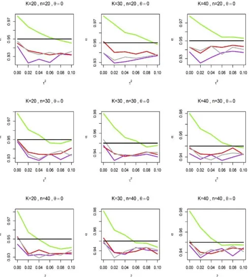
A desired estimator of 𝜏2 is the estimator that yielded a coverage probability of 𝜃 that is closer to the nominal level. Figure 1 shows
the coverage probabilities of 𝜃 produced based on estimators of
𝜏2 by DerSimonian and Laird (1986), Paule and Mandel (1982), Sidik and Jonkman (2005) and restricted maximum likelihood estimate (𝐷𝐿, 𝑃𝑀, 𝑆𝐽, 𝑎𝑛𝑑 𝑅𝐸𝑀𝐿) when 𝜃 = 0. For smaller
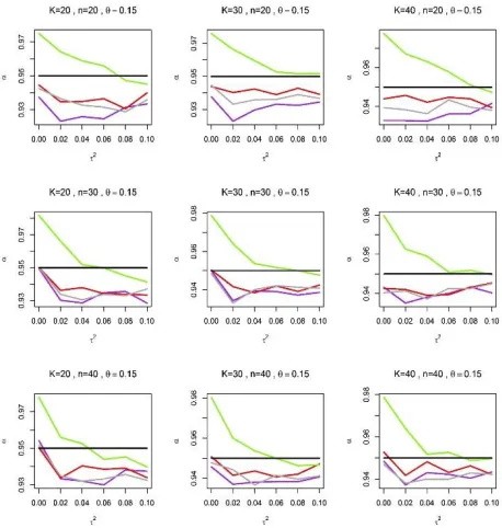
values of 𝜏2, coverage probabilities produce by 𝑅𝐸𝑀𝐿 are unsatisfactory, and are substantially far above the nominal level. Similar behaviour is also observed in Figure 2 when 𝜃 = 0.15. However as the values of 𝜏2 increased, the coverage probabilities produce by 𝑅𝐸𝑀𝐿 gradually improve, and eventually tends to the nominal level.
On the other hand, 𝐷𝐿, 𝑃𝑀, 𝑎𝑛𝑑 𝑆𝐽 yielded coverage
probabilities that generally fall below the nominal level. It is important to note that the coverage probabilities produced by these estimators are better compared to 𝑅𝐸𝑀𝐿 when 𝜏2≤
0.03. Although there is no much difference between the coverage probabilities yielded by 𝐷𝐿, 𝑃𝑀, 𝑎𝑛𝑑 𝑆𝐽, the coverage probability of 𝐷𝐿 is unsatisfactory when 𝜏2= 0.02, with coverage lower as 93%, far below the nominal level of 95%.
In summary, we can conclude on the basis of simulations that
𝑅𝐸𝑀𝐿 yielded the most accurate coverage probabilities when
effect estimates are substantially heterogeneous.
Figure 1: The coverage probability, 𝛼 of the population treatment effect 𝜃 calculated based on DerSimonian and Laird (1986), Paule and Mandel (1982), Sidik and Jonkman (2005) and the restricted maximum likelihood (𝐷𝐿, 𝑃𝑀, 𝑆𝐽, 𝑎𝑛𝑑 𝑅𝐸𝑀𝐿) estimators of 𝜏2 against 𝜏2 when 𝜃 = 0.
𝐷𝐿, 𝑃𝑀, 𝑆𝐽 𝑎𝑛𝑑 𝑅𝐸𝑀𝐿 are represented by purple, red, darkgray and chartreuse lines, respectively, and the black line represent the nominal coverage probability is set at 95%. 𝐾 is the number of studies for each meta-analysis and 𝑛 is the average sample size of studies.
Figure 2: The coverage probability, 𝛼 of the population treatment effect 𝜃 calculated based on DerSimonian and Laird (1986), Paule and Mandel (1982), Sidik and Jonkman (2005) and the restricted maximum likelihood (𝐷𝐿, 𝑃𝑀, 𝑆𝐽, 𝑎𝑛𝑑 𝑅𝐸𝑀𝐿) estimators of 𝜏2 against 𝜏2 when 𝜃 = 0.15.
𝐷𝐿, 𝑃𝑀, 𝑆𝐽 𝑎𝑛𝑑 𝑅𝐸𝑀𝐿 are represented by purple, red, darkgray and chartreuse lines, respectively, and the black line represent the nominal coverage probability is set at 95%. 𝐾 is the
number of studies for each meta-analysis and 𝑛 is the average sample size of studies.
Figure 3: The coverage probability, 𝛼 of the population treatment effect 𝜃 calculated based on DerSimonian and Laird (1986), Paule and Mandel (1982), Sidik and Jonkman (2005) and the restricted maximum likelihood (𝐷𝐿, 𝑃𝑀, 𝑆𝐽, 𝑎𝑛𝑑 𝑅𝐸𝑀𝐿)
estimators of 𝜏2 against 𝜏2 when 𝜏2= 0.08.
𝐷𝐿, 𝑃𝑀, 𝑆𝐽 𝑎𝑛𝑑 𝑅𝐸𝑀𝐿 are represented by purple, red,
darkgray and chartreuse lines, respectively, and the black line
represent the nominal coverage probability is set at 95%. 𝐾 is the number of studies for each meta-analysis and 𝑛 is the average sample size of studies.
On the other hand, 𝐷𝐿, 𝑃𝑀, 𝑎𝑛𝑑 𝑆𝐽 yielded better coverage probabilities compared to 𝑅𝐸𝑀𝐿 when treatment effects are homogeneous or moderately heterogeneous, although the coverage yielded by the three estimators are generally below the nominal level.
Summary and Conclusion
The main objective in meta-analysis is to combine results from different independent studies in order to obtain an accurate estimate of treatment effect and provide evidence base for decision making. There are two models, fixed-effect and random-effects models use to combine results in meta-analysis. Of the two models, random-effects model is the most widely use, see Hunter and Schmidt (2000), due to its ability to account for variation expected due to treatment effects or studies difference. This additional variability to the sampling variability is called the heterogeneity 𝜏2, which quantify the degree of inconsistency among the treatment effects. There are different ways to estimate
𝜏2, see Veroniki et al. (2015), and each of the methods differs in terms of precision and bias in estimating 𝜏2. In Section 2, the estimate of the population treatment effect in REM, 𝜃̂𝑅𝐸𝑀 is a function of 𝜏2, therefore the choice of the estimator of 𝜏2 is a crucial issue in random-effects meta-analysis.
This paper compares the effect of four estimators by DerSimonian and Laird (1986), Paule and Mandel (1982), Sidik and Jonkman (2005) and the restricted maximum likelihood method (𝐷𝐿, 𝑃𝑀, 𝑆𝐽, 𝑎𝑛𝑑 𝑅𝐸𝑀𝐿) on random-effects meta-analysis. In particular, the paper seeks to identify which of the estimators considered yields an accurate coverage probability for the population treatment effect 𝜃. Simulations reveal that each of the estimators considered leads to different coverage probability for
𝜃. 𝑅𝐸𝑀𝐿 estimator yielded the most accurate coverage probability for large values of 𝜏2. This result is consistence with the findings in Viechtbauer (2007) that of all estimators, the
𝑅𝐸𝑀𝐿 possess the properties in estimating 𝜏2 when the treatment effects are highly heterogeneous. In contrast to
𝑅𝐸𝑀𝐿, 𝐷𝐿, 𝑃𝑀, 𝑎𝑛𝑑 𝑆𝐽 perform better for smaller and moderate vales of 𝜏2. Therefore, the restricted maximum likelihood estimator of 𝜏2 is recommended for use in random-effects meta-analysis when treatment random-effects are highly heterogeneous, while any of the estimators by DerSimonian and Laird (1986), Paule and Mandel (1982) and Sidik and Jonkman (2005) can be used for homogeneous and moderately heterogeneous treatment effects.
The observed effect estimates use in the simulations were generated based on normality assumption. However, approximate normality of treatment effects only holds when effect estimates are sample means or mean difference. For other effect measures such as binary effects, normality of the distribution of the effect estimates only holds true when the sample sizes of studies are large, which is not often attainable in practice. For this reason, further investigation on the effect of estimators of 𝜏2 given different effect size on random-effect meta-analysis is recommended. Another important statistical tool recommended for such an investigation is the use of mean square error (mse).
REFERENCES
Biggerstaff, B. and Tweedie, R. (1997). Incorporating variability in estimates of heterogeneity in the random-effects model in meta-analysis. Statistic in medicine, 16(7):753-768.
DerSimonian, R. and Kacker, R. (2007). Random-effects model for meta-analysis of clinical trials: an update.
Contemporary clinical trials, 28(2):105-114.
DerSimonian, R. and Laird, N. (1986). Meta-analysis in clinical trials. Contemporary clinical trials, 7(3):177-188.
Dogo, S. H. (2016). Some statistical problems in sequential meta-analysis. PhD thesis, University of East Anglia, United
Kingdom.
Glass, G. V., McGaw, B. and Smith, M. L. (1984). Meta-analysis in social research. Sage Newbury Park.
Hedges, L. V. (1987). How hard is hard science, how soft is soft science? The empirical cumulativeness of research.
American Psychologists, 42(5):443.
Hedges, L. V. and Vevea, J. L. (1998). Fixed- and Random-effects models in meta-analysis. Psychological methods, 3(4):486.
Hoaglin, D. C. (2016). Misunderstanding about Q and Cochran’s Q test in meta-analysis. Statistics in medicine, 35(4):485-495.
Hunter, J. E. and Schmidt, F. L. (2000). Fixed effect vs random-effects meta-analysis models: implication for cumulative research knowledge. International Journal of Selection
and Assessment, 8(4):275-292.
Paule, R. C. and Mandel, J. (1982). Consensus values and weighting factors. Journal of Research of the National
Bureau of Standards, 87:377-385.
Rosenthal, R. (1978). How often are our numbers wrong? American psychologist, 33(11):1005.
Schmidt, F. L. (1992). What do data really mean? Research findings, meta-analysis, and cumulative knowledge in psychology. American psychologist, 47(10):1173.
Sidik, K. and Jonkman, J. N. (2005). Simple heterogeneity variance estimation for meta-analysis. Journal of the
Royal Statistical Society: Series C (Applied Statistics),
54(2):367-384.
Sutton, A. J., Abrams, K. R., Jones, D. R., Sheldon, T. A., and Song, F. (2000). Methods for meta-analysis in medical
research, volume 1, Wiley Chichester.
Term, H. (2002). Descriptive statistics for research. Institute for
the Advancement of University Learning, Department of Statistics, University of Oxford.
Veroniki, A. A., Jackson, D., Viechtbauer, W., Bender, R., Bowden, Knapp, G., Kuss, O., Higgins, J., Langan, D., and Salanti, G. (2015). Methods to estimate the between-study variance and its uncertainty in meta-analysis.
Research Synthesis Methods.
Viechtbauer, W. (2005). Bias and efficiency of meta-analytic variance estimators in the random-effects model. Journal
of Education and Behavioural Statistics, 30(3):261-293.
Viechtbauer, W. (2007). Confidence intervals for the amount of heterogeneity in meta-analysis. Statistics in medicine, 26(1):37-52