TR-IMDEA-Networks-2012-1
SOLOR: Self-Optimizing WLANs
with Legacy-Friendly
Opportunistic Relays
Andres Garcia-Saavedra
Balaji Rengarajan
Pablo Serrano
Daniel Camps-Mur
Xavier Pérez-Costa
SOLOR: Self-Optimizing WLANs with
Legacy-Friendly Opportunistic Relays
Andres Garcia-Saavedra
∗, Balaji Rengarajan
†, Pablo Serrano
∗, Daniel Camps-Mur
‡, Xavier P´erez-Costa
‡∗University Carlos III, Madrid, Spain †Institute IMDEA Networks, Madrid, Spain ‡NEC Network Laboratories, Heidelberg, Germany
Abstract—Current IEEE 802.11 WLANs suffer from the well-known rate anomaly problem, which can drastically reduce network performance. Opportunistic relaying can address this problem, but three major considerations, typically considered separately by prior work, need to be taken into account for an efficient deployment in real-world systems: 1) relaying could imply increased power consumption, and nodes might be hetero-geneous, both in power source (e.g., battery-powered vs. socket-powered) and power consumption profile; 2) similarly, nodes in the network are expected to have heterogeneous throughput needs and preferences in terms of the throughput vs. energy consumption trade-off; and 3) any proposed solution should be backwards-compatible, given the large number of legacy 802.11 devices already present in existing networks.
In this paper, we propose a novel framework, Self-Optimizing, Legacy-Friendly Opportunistic Relaying (SOLOR), which jointly takes into account the above considerations and greatly improves network performance even in systems comprised mostly of vanilla nodes and unmodified access points. SOLOR jointly optimizes the
topology of the network, i.e., which are the nodes associated to each relay-capable node; and the relay schedules, i.e., how the relays split time between the downstream nodes they relay for and the upstream flow to an access point. The results, obtained for a large variety of scenarios and different node preferences, illustrate the significant gains achieved by our approach. Its feasibility is demonstrated through test-bed experimentation in a realistic deployment.
I. INTRODUCTION
In IEEE 802.11 WLANs, stations associated to an Access Point (AP) can experience different signal-to-noise ratios (SNRs), depending on several factors, e.g., their distance to the AP, the presence of physical obstacles, or the particular characteristics of their RF equipment. The various physical layers available (see [1] for a survey of existing 802.11 standards) offer stations a variety of modulation and coding schemes (MCS) to choose from, in order to optimally adapt the MCS to the channel conditions. However, it is well-known that this heterogeneity in the use of MCS may induce therate
anomaly problem [2], which degrades the performance of the
WLAN.
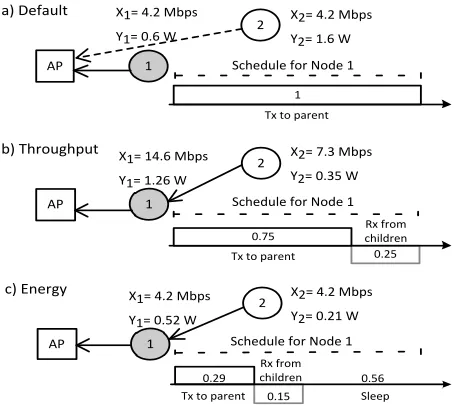
To illustrate the above, let us consider the case of uplink traffic in the toy scenario of Fig. 1a, which we refer to as the “Default” case and that consists of two stations (nodes 1 and 2) simultaneously transmitting to an AP. Given their different radio conditions, node 1 uses the 48 Mbps rate, while node 2 uses 6 Mbps. In this case, both stations will receive equal
0.25
0.15
0.29 0.56
Tx to parent Sleep
Rx from children
AP 1
2
a) Default X2= 4.2 Mbps
Y2= 1.6 W
1
Tx to parent
Schedule for Node 1 X1= 4.2 Mbps
Y1= 0.6 W
AP 1
2
b) Throughput X2= 7.3 Mbps
Y2= 0.35 W
0.75
Tx to parent
Schedule for Node 1 X1= 14.6 Mbps
Y1= 1.26 W
Rx from children
AP 1
2
c) Energy X2= 4.2 Mbps
Y2= 0.21 W Schedule for Node 1 X1= 4.2 Mbps
Y1= 0.52 W
Fig. 1. Different configurations for a deployment consisting of one AP and two stations (one with relay capabilities, marked in grey).
throughput of approximately X1 =X2 = 4.2 Mbps,1 which
for the case of node 1 is well below its maximum achievable rate. This phenomenon is termed the rate anomaly problem, and is a direct consequence of the medium access mechanism, which results in the station transmitting at low rate occupying the channel for the majority of time.
A method that has been proposed to address this rate anomaly problem, and in general to lessen the impact of poor radio conditions, is to use the relaying capabilities of some nodes [3]–[8] (related work is discussed in detail in Section VI), which can act as APs for those suffering from poor radio conditions. Indeed, this opportunistic use of the “AP-like” functionality has been defined in the Wi-Fi Direct specification [9], which is readily available in several devices (e.g., recent Android phones), some of them building on the p2p2 open-source implementation.
For example, in our toy scenario, if node 1 is relay-capable, it could enable the cases of Fig. 1b and Fig. 1c, which we name as “Throughput” and “Energy”, respectively, for reasons that will become evident shortly. In these cases, node 1 acts as an AP for node 2, and is responsible for sending both its own
1The model used to compute the throughput and power consumption figures is detailed in Section II.
2
data and that of node 2 to the AP. This creates a different topology, i.e., the paths between stations and the AP (we will formally introduce our terminology in the next section). Assuming that nodes are equipped with a single radio, node 1 has to time share between serving node 2 and transmitting to the AP. We refer to this choice of the fractions of time a relay spends in these activities as the relay schedule. Given the new topology considered in the figure, the schedule will determine the network performance, and therefore it has to be tuned depending on some optimization criterion.
For the case of Fig. 1b, the network is optimized based exclusively on throughput considerations, and according to
the proportional fairness criterion, which results in node 1
spending 25% of its time serving node 2, and the rest of the time transmitting to the AP. Clearly, even in this fairly sim-ple scenario, the throughput improvements obtained through the intelligent use of relaying can be significant. However, although all nodes get higher throughput, now the power con-sumption of the relay (Y1) is higher than in the Default case,
due to the increased time spent in energy-intensive operations, i.e., transmitting and receiving packets. With mobile, battery-powered devices being sensitive to energy consumption, this trade-off between performance and energy consumption has to be carefully managed [10]. An alternate relay schedule, which minimizes energy consumption (by making use of sleep modes) while guaranteeing minimum throughput above the Default scenario, is given in Fig. 1c. Here, node 2 is forced to sleep for 85% of the time, while node 1 sleeps for 56%, thus reducing the overall energy consumption from 2.20 W to 0.73 W (i.e., a 67% reduction).
The relative importance of throughput and power con-sumption depends on the characteristics of each station, e.g. whether it is battery-powered or plugged in to a socket, the throughput requirements of the application, and so on. The criterion used, and the topology and schedule chosen should reflect the preferences of the nodes in the network. Another important consideration from the point of view of practicality is backwards-compatibility. Given the large number of legacy 802.11 devices already present in existing networks, mecha-nisms that require changes in all nodes in order to work are impractical. A practical scheme must be able to work under the distributed coordination function (DCF), which is the most prevalent operating mode in existing 802.11 networks. As we show in the sequel, significant performance gains and power savings can be obtained even when the ratio of relay-capable nodes to legacy nodes is low.
The key contributions of this paper are:
• A novel, legacy-friendly framework for optimization of performance and power consumption of a WLAN with relay-capable nodes, reflecting heterogeneous power vs. performance preferences of individual nodes.
• A low-complexity algorithm for topology control, that enables the joint optimization of network topology and relay schedule in a fast, scalable manner.
• Numerical evaluation for a large variety of scenarios in terms of node density, proportion of relays, network size,
and performance criteria that illustrate the flexibility and benefits of the proposed framework.
• Experiments using a real-world testbed comprised of off-the-shelf devices that demonstrate the practicality of the proposed approach and validate the model and the achieved gains.
The rest of the paper is organized as follows. In Section II we introduce the key parameters of our model, namely, topol-ogy and relay schedule, and present the throughput and power consumption models used throughout the paper. In Section III we present our optimization framework that can be solved for the optimal relay schedule and heuristics to pick the best topology. The results from the optimization are provided in Section IV for a variety of WLAN deployments, while in Section V we report our experimental results using a mid-sized testbed composed of commercial, off-the-shelf devices. Related work is discussed in Section VI. Finally, Section VII summarizes our contributions and concludes the paper.
II. SYSTEMMODEL ANDNOTATION
Our scenario consists of a network with one AP, denoted node 0, andN other nodes, together denoted by the setN =
{0,1,2, . . . , N}. LetS ⊆ N be the set of relay-capable nodes, which for notational convenience includes the AP. We assume that all nodes are single-radio, i.e., they cannot simultaneously transmit over two different channels. We focus, for simplicity, on the uplink case and assume that all nodes are saturated, i.e., their buffers are always backlogged. We denote by Rij, the
rate corresponding to the MCS used between nodes i, j, and withRi the data rate of the MCS at which nodeitransmits to
the AP, i.e.,Ri:=Ri0. The channels used for communication
between the AP/relays and their corresponding stations are chosen such that they do not interfere with each other.
A. System Abstractions
Network Topology: We assume that each node uses only one
path, consisting of one or more wireless links, to reach the AP (i.e., no multi-path). We refer to thetopologyof the network as the set of paths that nodes use to reach the AP. More formally, the network topology is specified by defining for each noden,
itsparent An∈ S, which is the first-hop node on the path to
the access point. For the case of e.g. Fig. 1b, the topology is defined as{A1= 0, A2= 1}. Given a topology{An}, we can
determine for each nodem∈ N its set ofchildrenCm, i.e., the
set of nodes one hop away frommthat reaches the AP through it, asCm={n:n∈ N, An=m}. The complete set of nodes
that usemto reach the AP is defined asTm=Cm
S
n∈ CmTn. Note that, for a nodem /∈ S,Tm=Cm=∅.
Relay Schedule: A relay-capable node can, in general, be in
0.15 0.2
AP
1
2
3
0.35 0.65
Tx to parent Sleep
Schedule for Node 1
Tx to
parent Sleep
Rx from children
Schedule for Node 3
0.1 0.4
0.15 Tx to
parent
Rx from children
18Mbps
6Mbps
48Mbps 48Mbps
48Mbps
48Mbps
F0 {1}
F0 {1,3}
AP fractions
F0
{3} F 0
{}
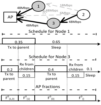
Fig. 2. Scenario with two relays and one client.
node 3 are relay-capable. Here, node 3 spends part of the time transmitting to the AP, and part of the time acting as AP for node 2. We denote by Ws the collection of all possible
sets of nodes that could simultaneously transmit to a given relay s. For the case of Fig. 2, we have W3 = {(2)} and
W0 = {(1,3),(1),(3)} (note that node 1 is also a
relay-enabled node). Fig. 2 also illustrates that the relay schedules determine the fraction of time that a particular set of nodes V ∈Wsis simultaneously transmitting to relays. For the case
of the AP, we have that e.g. it receives traffic from nodes 1 and 3 for 20% of the time, which we denote asF0
{1,3}= 0.2, and it
does not receive traffic from any node 25% of the time, which is denoted asF0
{} = 0.25. As we will detail in Section III, the
policy that we follow to compute the relays’ schedules ensures a one-to-one mapping between these and the set of fractions
~ F ={Fs
V;s∈ S,V ∈Ws}.
The configurationof the network is jointly determined by the topology {An} and the relay schedules with the induced
set of fractionsF~.
B. Throughput model
LetRsV(n)be the throughput obtained by noden∈ V from relay s when the set of nodes simultaneously transmitting to s is V. This can be computed by following, for example, our analysis in [11] that extends the seminal work of [12] to address heterogeneous MCS. We will use the convention thatRs
V(n) = 0ifn /∈ V. In the sequel, we suppress the relay
identity, s. Based on this, the total throughput obtained by a non-relay node nis computed as the average throughput over time as:
Xn =
X
V∈WAn
RV(n)FAn
V . (1)
In order to compute the throughput of a relay node s ∈ S\{0}we need to subtract from the total throughput it obtains, the throughput required to serve the set of nodes that access the AP through it (i.e., Ts),
Xs=
X
V∈WAs s∈V
FAs
V RV(s)−
X
t∈Ts
Xt. (2)
C. Power Consumption Model
We follow the conventional model (see e.g. [13] and refer-ences therein) that the power consumption of an 802.11 node can be modeled after the fraction of time it spends in transmit, receive, idle, and sleep modes, along with the corresponding per-state power consumption figures (see [14] for an extensive survey of thses). We denote by PT
V(n) the power consumed
by node n when the set of active nodes transmitting to its relay isV. Here, the dependence on V, the set of contending nodes, reflects the effect of contention, and the frame spacings mandated by the 802.11 standard. The above can be computed by following, for example, our results in [13]. We will assume that whenever a node is not actively transmitting data because its parent is not available, it remains in the sleep state with corresponding power consumption ρs.3 Based on this, the
power consumed by a non-relay node n /∈ S is computed as
Yn=
X
V∈WAn FAn
V PVT(n) + (1−
X
V∈WAn FAn
V )ρs. (3)
Similarly, we denote with PVR(s) the power consumed by relayswhen receiving traffic from the setVof children, which again can be computed following [13]. Hence, the power consumption of a relay nodes∈ S \ {0} is given by:
Ys=
X
V∈WAs s∈V
FAs
V PVT(s) +
X
V∈Ws
FVsPVR(s)
+ (1− X
V∈WAs s∈V
FAs
V −
X
V∈Ws FVs)ρs.
III. COMPUTING THEOPTIMALCONFIGURATION
We propose SOLOR, a utility-based framework for opti-mizing the configuration of the WLAN. We compute the total utility of a nodenthat obtains a throughputXnand consumes
Yn as Un(Xn)−Ln(Yn). Here, Un(·) is a concave function
that maps user n’s throughput to a utility, and Ln(·) is a
convex function that maps the energy consumption of user n to an incurred cost. For example, the energy cost could model the effect on the user of the implied reduction in battery lifetime. Both the concave nature of the energy cost and the throughput utility functions derive from the common assumption of diminishing marginal returns [15]. We divide the problem of optimizing network configuration into two parts, i.e., optimizing the relay schedule and choosing the best network topology. We first present a convex program that, given a network topology and a set of users’ preferences, com-putes the optimal relay schedule. Next, we describe different approaches that leverage the above convex optimization to find the topology that aims at optimizing performance.
4
A. Computing the Optimal Relay Schedule
We frame the problem of choosing the optimal relay sched-ule in terms of choosing a feasible set of fractions F~ that maximizes overall utility as follows:
max
~ F
N
X
n=1
U(Xn)− N
X
n=1
Ln(Yn) (4a)
subject to Xn≥0,1≤n≤N (4b)
N
X
n=1
Xn≤C (4c)
Xn≥xminn (4d)
Yn ≤ymaxn (4e)
Un(Xn)−Ln(Yn)≥dn,1≤n≤N (4f)
0≤FVs≤1,∀s∈ S,∀V ∈Ws (4g)
X
V∈W0
FV0≤1 (4h)
X
V∈WAs s∈V
FAs
V +
X
V∈Ws
FVs≤1,∀s∈ S (4i)
Objective function (4a) is the sum utility of all the nodes in the network, which can be tailored to different optimization problems as we briefly discuss below. Equations (4b) and (4c) constrain that the throughput figures take values between zero and a maximum backhaul capacityC. The constrains (4d)–(4f) support setting per-node preferences, while (4g)–(4i) ensure that the chosen fractions of time are feasible, i.e., that the valid schedule that induces these fractions exists.
Setting per-node preferences. Eq. (4d) specifies a per-node lower bound on the throughput of a per-node and thus is a lower bound on performance, while (4e) specifies an upper limit on the amount of power each node is willing to expend. Eq. (4f) specifies the trade-off between energy consumption and performance that is acceptable to each node. When a node chooses dn → −∞, the node is collaborative, willing
to sacrifice its individual utility in order to maximize the overall utility (for example, in a home network where all the devices share an owner, this might be appropriate). More subtle preferences are also supported, e.g., setting dn equal to the
utility of the node in the default case imposes the constraint that every node must benefit from the relay-based setup.
Computing a feasible set of fractions. Eqs. (4g)–(4i) guarantee that the fractions chosen are such that, from the point of view of any relay or the AP, the total fraction of time it is required to stay connected to either its children or parent is less than one and thus achievable. The first term on the left hand side of constraint (4i) is the fraction of time relay s is connected to its parent, and the term on the right hand side is the fraction of time it serves its children. Note that a relay spends the time that it is neither transmitting or receiving, i.e., the gap in constraint (4i), in sleep mode. Given a feasible set of fractions, F, many compliant schedules can potentially~ be constructed. We describe below, a deterministic policy to construct a schedule consistent with a given set of fractions
that demonstrates clearly that a set of fractions satisfying the above constraints is indeed realizable.
Mapping time fractions to relay schedules.We compute the schedules of the relays starting from those one hop away from the AP, and then moving one hop at a time (the schedules of relays that share the same path length to the AP can be computed in any order). For each relay s∈ S, we impose a deterministic ordering of the sets in Ws (for example, one
based on the size of the set and using the smallest node identifier, e.g., MAC address, as a tiebreaker). We start by arranging the fractions F0
V,V ∈W0 in the order determined
by the ordering imposed on W0. This specifies exactly, the
time periods when the children of the AP have to contend for access to the relay. Next, for each relaysthat is one hop from the AP, we determine the rest of its schedule by splitting the time thatsis not sending to the AP into the time fractionsFVs. Again the ordering of the fractions is the same as that imposed onWs. Note that the time left over is the fraction of time relay s spends in sleep mode and always occurs at the tail of the sequence of time fractions. In this manner, we can continue increasing the path length, with the fractions corresponding to a relay specifying a part of the children’s schedule, i.e., the time period when they contend for access to the relay.
B. Computing the Relay Topology
Given a topology, the optimization problem above deter-mines the optimal relay schedule. Here, we focus on the problem of computing the relay topology that maximizes overall network utility. In general, this is a combinatorial problem, and efficiently finding the optimal topology does not appear to be possible as the decision of a single node to switch its parent could affect the throughput that can be achieved by all the nodes in the network. We consider three possible approaches to the topology selection problem with varying degrees of complexity:
Brute Force:This algorithm simply testsallvalid network topologies, solving the optimization problem 4 for each topol-ogy, and choosing the topology that maximizes the overall utility. For large networks, especially those with many relays, this approach is not computationally tractable. However, since this brute force search is guaranteed to find the globally optimal solution, we use it to benchmark the other heuristics. Closest-first:In this simple heuristic, each node associates to the relay to which it has the highest MCS, irrespective of the set of nodes that are connected to that relay, or the quality of the channel between the AP and the relay. Once the topology is chosen, the optimization problem is solved once in order to configure the network. As compare to the previous scheme, this heuristic is extremely simple, but does not take into account the interactions between various key variables of the WLAN.
A greedy algorithm: This is a heuristic aiming at
node changes its parent; the heuristic solves the optimization problem for each of these alternatives and picks the topology that maximizes the utility. Note that the utility is bounded, and since the overall utility increases monotonically as the heuristic progresses, it is guaranteed to converge. In the sequel, we demonstrate that this approach achieves utilities that are very close to optimal.
C. Different Optimization Criteria
The optimization problem maximizes a concave objective function under a convex set of constraints and thus admits a unique optimum. The SOLOR framework can be used to model a number of scenarios depending on the subset of constraints that are included and the choices of the utility functions and the energy cost function, as we will demonstrate in the sequel. For example, consider omitting constraints (4d) - (4c), and setting Ln(Yn) = 0,∀n. Proportional fairness
could be modeled by choosing logutility functions, and max-min fairness (when achievable) could be achieved by setting Un(Xn) =Xn,∀nand adding the constraints:Xn =X1,∀n.
In the rest of the paper, unless noted otherwise, we focus on scenarios where utility functions are of the form:
Un(Xn) =αnlog(Xn)
Ln(Yn) = (1−αn)Yn,
whereαnmodels the per-node priorities of power consumption
vs. performance (a high value of αn prioritizes performance
over power consumption and vice-versa).
D. Bi-Directional Traffic
Note that while we focus on the case of uplink traffic for simplicity, the above problem formulation can also be used to model the scenarios with bi-directional traffic. In this case, utility function could be defined separately for each of the uplink and downlink flows. In each time fraction Fs
V that we
consider, there would be both uplink and downlink traffic, and a throughput model similar to the one defined in Sec. II can be used to calculate the throughput of both the uplink and downlink flows. Here, we would have to separately define the average uplink and downlink rates received by a node in each time fraction, i.e., we would have to replace the rates RV(n)
with the uplink and downlink versions RUL
V (n) and RDLV (n).
The above rates could still be calculated using [11] with the AP/relay being another contending node in the network. The power consumption model would have to be similarly modified.
IV. PERFORMANCEEVALUATION
In this section we quantify the performance improvements that can be achieved using SOLOR. The simple case of a network with two nodes, one with relay capabilities, has already been discussed in Section I (this was the only case considered in [4]). In what follows, we first analyze the case of a two-relay network like the one depicted in Fig. 2, with homo-and heterogeneous per-node settings for the performance vs. energy trade-off, and then address the case of random topolo-gies with larger number of nodes and relays.
0 5 10 15 20 25 30
0 1 2 3 4 5
Throughput (Mbps)
Power (Watts)
a) Single-hop
0 5 10 15 20 25
Thr Pwr Default
Thr Pwr energy optimal
Thr Pwr Max-Min
Thr Pwr PF α=1
Thr Pwr PF α=0.25
0 1 2 3 4
Throughput (Mbps)
Power (Watts)
b) Multi-hop Relay 3 Relay 1 Node 2
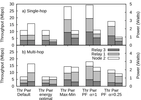
Fig. 3. Improvements for the two-relay scenario for different optimization criteria
A. A two-relay, three node network of homogeneous nodes
Single-hop relaying: We first consider the scenario illus-trated in Fig. 2, in which nodes 1 and 3, both with relays capabilities, can transmit to the AP atR1 =R3= 48 Mbps.
Node 2 can transmit to the AP at R2 = 6 Mbps, and
could send traffic to nodes 1 and 3 at R21 = 18 Mbps and
R23= 48Mbps, respectively. We first obtain, as a benchmark,
the (equal) throughput,X(def ault), achieved by each node in the “default” case, i.e., when all nodes directly transmit to the the AP. We analyze the performance of the SOLOR framework under the following optimization criteria:
• The “energy-optimal” configuration, obtained by setting αi= 0∀i andxminn =X(def ault).
• The “max-min” optimal configuration, i.e., maximizing the lowest individual throughput.
• The “proportional-fair” (PF) configuration, without en-ergy considerations (αi = 1∀i) and with energy
consid-erations (αi= 0.25∀i).
Note that the topology chosen by our framework is identical to the one depicted in Fig. 2 in all the cases, and also coincides with the optimal topology.
Fig. 3a depicts the throughput and power consumption of each node in the different settings. The results demonstrate the gains that can be achieved by SOLOR along the two dimensions of interest, depending on the preferences of the nodes. For example, in the case of PF with no energy considerations, the overall throughput increases by 170%, with each node benefiting substantially (note that the share is almost purely fair). However, in this case, node 3 acting as the relay for node 2 does consume higher power than in the default scenario. When the nodes are highly energy constrained, SOLOR enables power savings of 74% without any of the nodes sacrificing throughput.
Multi-hop relaying: To demonstrate the effectiveness of SOLOR in scenarios that call for multi-hop relay topologies, we consider the network in Fig. 2, with the link from node 3 to the AP degraded to R3= 6 Mbps, emulating for example
6
all the settings considered (and the one chosen by SOLOR) is one in which node 3 accesses the AP through node 1 at R13 = 48 Mbps while continuing to relay for node 2.
The results for this scenario are depicted in Fig. 3b, and show the same qualitative behavior as in the earlier case. The raw throughput (and power savings) achieved, in this more hostile environment, is not as high as in the earlier scenario, however the gain over the default case is still significant (160% throughput increase under PF, and 60% energy savings in the energy-optimal case).
B. A two-relay, three node network of heterogeneous nodes
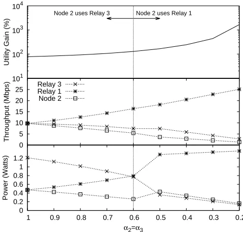
One of the key features of SOLOR is its ability to support individual node preferences. We explore the effect of the parameterαand the ability of SOLOR to adapt, focusing from this point forward on the PF criterion. We consider again the WLAN depicted in Fig. 2 without the obstacle between node 3 and the AP, and assume that node 1 is not power constrained (e.g., connected to a wall socket) and thus has α1 = 1. We
examine a range of scenarios where the sensitivity of nodes 2 and 3 to power consumption progressively increases as they become increasingly power constrained (mobile devices).
Fig. 4 depicts the gain achieved by SOLOR over the default scenario as the value of α2 = α3 increases. The results
demonstrate that SOLOR is able to adapt to different per-node preferences on the trade-off between power and throughput. Indeed, Fig. 4 illustrates that when throughput performance is critical, and nodes 2 and 3 prioritize throughput over power savings, the topology chosen is the one illustrated in Fig. 2 that favors higher throughput (R21 < R23). However, as node 3
becomes increasingly power constrained, the topology chosen switches to one in which node 2 reaches the AP through node 1, as shown in Fig. 4, enabling node 3 to save power. Note that in the power hungry scenarios, the gain achieved by SOLOR explodes as nodes are able to obtain their desired throughput in a highly energy-efficient manner.
C. Random network topologies with multiple relays
Finally, we analyze the performance improvements of SOLOR in random topologies consisting of different number of nodes and relays. The generation of a random deployment consist of the following steps: (i) we assume a square area of size 20 m×20 m, in which the AP is located in one of the corners; (ii) we randomly deploy N nodes in the area, following a 2-D Gaussian distribution centered on the AP and with σ = 10 m (if a node falls outside the considered area, it is re-deployed).4(iii) we randomly pick R out of the
N nodes, as being relay-capable; (iv) finally, based on the distances between nodes (we apply the log-distance path loss model with shadowing parametrized for an office environment with hard partitions [18]), we use the MCS vs. SNR curves
4Although there are well-known random generators available, such as the Hyacinth-Laca tool used in e.g. [16], [17], these are typically used for the case of large muti-hop wireless (mesh) networks, while our focus is on smaller-sized deployments.
101 102 103 104
Utility Gain (%)
Node 2 uses Relay 3 Node 2 uses Relay 1
0 5 10 15 20 25
Throughput (Mbps)
Relay 3 Relay 1 Node 2
0 0.2 0.4 0.6 0.8 1 1.2
0.2 0.3 0.4 0.5 0.6 0.7 0.8 0.9 1
Power (Watts)
α2=α3
Fig. 4. WLAN performance for the deployment of Fig. 2 and different configurations ofα2,3.
provided in [19] to obtain the transmission rates between each pair of nodes.
For each scenario, we first compute the WLAN performance for the “default” case, and then the performance when using SOLOR. We compare the performance of the three approaches to compute relay topology described in Section III-B, although the brute-force scheme is not computationally tractable for some scenarios. Indeed, in a WLAN deployment consisting of 6 nodes, 3 of them relays, performing an exhaustive search in the configuration space requires solving the convex problem almost 400 times, while our greedy scheme reduces this number to 60. In order to obtain statistically significant results, we generate as many random topologies as required to obtain 95% confidence intervals of 10%.
Impact of network size:We first analyze performance with varying number of nodes in the WLAN, when half of them are relay-capable. Like in the previous section, we stick to the PF optimization, for two different choices ofαn, namely,αn= 1
(indifferent to power saving) andαn= 1/7(sensitive to power
consumption). For each scenario we compute the gain in the overall utility as well as the gains in throughput and power consumption relative to the default case.
40 80 120 160
Utility Gain (%)
Brute Force Greedy Closest First
10 20 30 40
Throughput Gain (%)
0 5 10 15 20 25 30
2 4 6 2 4 6
Power savings (%)
Number of nodes α=1/7
α=1
Fig. 5. Performance improvements for different network sizes.
off between throughput performance and power consumption. Impact of relay density: Next, we analyze the performance of SOLOR as the proportion of relay-capable nodes changes, for topologies consisting of five nodes. The results are depicted in Fig. 6, and show that when the relative number of relays is low (1 out of 5), the performance improvements are low, a result that is not surprising as the relay is chosen by randomly picking one of the five nodes deployed, rendering it ineffective in most cases. Despite this, the results show that even when only two of the nodes are relay-capable, the performance improvement is significant (e.g., throughput gains around 20% for αn = 1), and these can grow up to
100% improvement in the case of all-relay networks. When α = 1/7, power savings on the order of 80% are achieved on average in all-relay networks while overall throughput performance is also improved by 20%. Finally, the results from the greedy algorithm are very similar to those from the brute-force approach, whose computational complexity is prohibitive for topologies with more than three relays (note that given our requirements on the size of the confidence interval, for these configurations we have to run more than 1000 random topologies).
The results in this section demonstrate the effectiveness of SOLOR in maximizing performance in very diverse heteroge-neous settings. In the next section, we describe a preliminary deployment of SOLOR in a real-life testbed consisting of seven machines that validates our findings.
V. EXPERIMENTALEVALUATION
Here we describe the results from a first implementation of the SOLOR framework. Our 802.11g testbed, represented in Fig. 7b, is comprised of seven nodes, all using Ubuntu 11.10 with kernel 3.00. There are four legacy nodes, one of which is the AP, and three relay-enabled nodes. The legacy nodes are standard laptops equipped with WLAN cards based on the Atheros AR5413 chipset, using the ath5k/mac80211 wireless subsystem, while the relay-capable nodes are desktop
20 40 60 80 100 120 140
Utility Gain (%)
20 40 60 80 100
Throughput Gain (%)
0 20 40 60 80 100
1/5 2/5 3/5 4/5 5/5 1/5 2/5 3/5 4/5 5/5
Power Savings (%)
Proportion of relays Brute Force
Greedy algorithm Closest-First
α=1/7 α=1
Fig. 6. Impact of the proportion of relays
(a) Software modules.
A B
C
T
o
p
lo
g
y
1 2 3
4 5 6
(b) Testbed deployed.
Fig. 7. Implementation architecture.
machines, each equipped withtwoWLAN cards based on the Atheros AR922X chipset and using the ath9k/mac80211 subsystem. We decided, for simplicity, to use two NICs to emulate a single NIC with the ability to serve as AP on one channel and to connect to an AP on a different channel, as existing open-source drivers do not support this feature yet.5 On the other hand, our implementation will not require any modification once this feature becomes available. Note that, throughout our experiments, we take great care in confirming that only one of the two NICs is active at any point in time.
A. Implementing SOLOR
In order to implement SOLOR, three main functionalities are required: a) to analyze the WLAN deployment and com-pute the optimal configuration; b) to implement the resulting relay schedules; c) to force legacy nodes to connect to the proper relay and to sleep when needed. This is achieved by the software architecture depicted in Fig. 7a, consisting of a
8
space application that computes the optimal configuration, and a kernel module (solor.ko) to interact with the Linux wireless subsystem.
SOLOR nodes obtain a vision of the network by sniffing wireless traffic, thus estimating the relative link qualities between nodes.6 Furthermore, given that in this section we
stick to the PF optimization with αn= 1, there is no need to
gather per-node preferences and characteristics (e.g., power consumption), which could be explicitly obtained with ad-hoc messaging or inferred based on, e.g., MAC addresses. The optimal configuration of the network is independently computed by each SOLOR node; given the policies described in Section III, using MAC addresses as node IDs, this will result in all relays computing the same joint schedule with fractions F. To implement this schedule, the~ solor.ko module builds on the synchronization provided by beacon frames sent by each parent, and triggers the corresponding notifications to the driver by sending them through mac80211. In order to force legacy nodes to de-associate from the AP and to connect to the relay, we use a simple scheme based on the behavior of the Ubuntu wireless network manager, which is common to other network managers. The scheme is based on the relay forging a disassociation message as if it were sent from the AP, thus forcing the legacy node to re-scan the entire network looking for the best AP to associate with for the pre-configured SSID. The relay will then announce itself as a better AP for that network (otherwise, the computed topology would worsen the overall performance), thus ensuring that the legacy node will associate with it. According to our measurements, this procedure takes between two and four seconds. Finally, we need to ensure that legacy nodes go to sleep or, at least, do not transmit while the relay is not available (either sleeping or sending data to its parent). Again, for simplicity, we decided to use theNotice of Absence (NoA) [9] protocol, specified for WiFi Direct and already present in many current devices (e.g. Android phones). We also tested other feasible schemes not relying on NoA, e.g., sending null data frames with a setting of the Network Allocation Vector equal to the time the AP is not available, which enables the node to sleep for that period of time (very-old NICs overhearing all traffic in the network will not go to sleep, but at least they will not transmit).
B. Validation and Performance Evaluation
Static conditions. We start our experimental evaluation by measuring the throughput performance of different static settings with a fixed topology, in order to validate the results from the previous sections. To this end, we consider the three topologies depicted in Fig. 7b and different settings of the transmission rate between the laptops and the relays (denoted as Rc), and the rates between the relays and the AP (denoted by
Rr), and compare the per-node throughput figuresXnobtained
in the testbed with the analytical ones. The results are depicted
6This simple scheme proves to be sufficiently accurate for our purposes, although in future developments we plan to implement a protocol to exchange these measurements, or to build on e.g. the 802.11k standard [1].
TABLE I
PER-NODE THROUGHPUT(INMBPS)FOR THE TOPOLOGIES INFIG. 7B.
Top. Rc, Rr X1,X2,X3 X4,X5,X6 (Mbps)
48, 48 14.60, -, - (14.62) 7.31, -, - (7.31) A 48, 24 14.22, -, - (14.62) 5.51, -, - (5.57) 24, 24 8.7, -, - (9.00) 4.65, -, - (4.5) 48, 48 7.46, 7.42, - (7.31) 6.98, 7.12, - (7.31) B 48, 24 7.64, 7.63, - (7.31) 7.16, 7.23, - (7.31) 24, 24 4.11, 4.92, - (4.50) 4.32, 4.10, - (4.50) 48, 48 5.30, 4.21, 4.42 (4.87) 3.80, 4.12, 3.84 (4.87) C 48, 24 4.53, 4.98, 4.41 (4.87) 4.30, 4.56, 4.52 (4.87) 24, 24 2.92, 3.22, 3.15 (3.00) 2.63, 2.52, 2.77 (3.00)
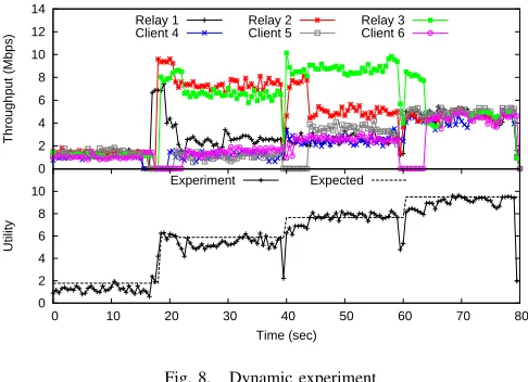
in Table I, showing that in all cases the experimental figures match remarkably well the results from the analytical model, which are provided in parenthesis (the same conclusions are obtained for different values ofαn, omitted for space reasons). Dynamic conditions. We next assess the performance of SOLOR in a dynamic scenario, in which nodes activate the relaying functionality in real-time and thus the topology changes over time. Nodes 1–3, which do not have the relay functionality activated at the beginning of the experiment, can transmit to the AP at 48 Mbps, while nodes 4–6 transmit to the AP at 6 Mbps, and could transmit to nodes 1–3 at 48 Mbps. Our experiment is divided in stages of approximately 20 seconds each. During the first stage, all nodes are transmitting to the AP, this being the “default” scenario; during the second stage, node 1 enables the SOLOR functionality and as a consequence starts relaying traffic for nodes 4–6; in the third stage, node 2 also enables the SOLOR functionality and relays the traffic from node 6, while node 1 keeps relaying for nodes 4 and 5; finally, in the last stage, node 3 is also enabled as a SOLOR node and, as a consequence, each relay-enabled node serves one client, i.e., the topology C depicted in Fig. 7b.
We display the evolution of the per-node throughput figures over time in Fig. 8 (top), in which the transient caused by the re-association periods can be easily identified. The corresponding overall utility of the WLAN is depicted in the bottom subplot, along with the theoretical values. We conclude from this experiment that enabling the relay functionality supports increasing the utility of the network, with a good match between experimental and analytical results, and that the SOLOR framework is easily implementable using commercial, off-the-shelf hardware.
VI. RELATEDWORK
Previously, the use of relays has been proposed to improve WLAN performance, based in most cases exclusively on throughput considerations and ad-hoc modifications to the standard behavior. For instance, in [3] the authors propose RAMA, an opportunistic relaying scheme where relay nodes
offerthemselves to other wireless nodes when there could be
0 2 4 6 8 10 12 14
Throughput (Mbps)
Relay 1 Client 4
Relay 2 Client 5
Relay 3 Client 6
0 2 4 6 8 10
0 10 20 30 40 50 60 70 80
Utility
Time (sec) Experiment Expected
Fig. 8. Dynamic experiment
Other proposals have been proposed with a specific appli-cation in mind, e.g., in [5] authors present PRO, a scheme that overhear frames and automatically re-transmit them on behalf of the sender whenever a loss is detected. Another application-tailored proposal is [6], in which a centralized scheme is presented to improve the delivery of multicast traffic within multicast groups.
In another related set of work, authors have analyzed the use of relays for energy efficiency. In [7], authors propose CoopMAC, a scheme where sending stations keep a list of relays with information on the delivery efficiency, and an extended MAC protocol that gives higher priority to relays is used. In [8] authors propose a centralized Cooperative Relay Service (CRS) for WLANs, where the AP is extended to act as a central coordinator that grants each station time to access the network
VII. CONCLUSIONS
In this paper we presented SOLOR a novel Self-Optimizing, Legacy-Friendly Opportunistic Relaying framework which ad-dresses therate anomalyproblem by taking into account three major considerations to achieve an efficient deployment in real-world systems: 1) relaying could imply increased power consumption, and nodes might be heterogeneous, both in power source (e.g., battery-powered vs. socket-powered) and power consumption profile; 2) similarly, nodes in the network are expected to have heterogeneous throughput needs and preferences in terms of the throughput vs. energy consumption trade-off; and 3) any proposed solution should be backwards-compatible, given the large number of legacy 802.11 devices already present in existing networks. SOLOR jointly optimizes
the topology of the network, i.e., which nodes associate to
each relay-capable node; and the relay schedules, i.e., how the relays split time between the downstream nodes they relay for and the upstream flow to an access point. The proposed framework has been evaluated considering a large variety of scenarios and different node performance/power consumption trade-off preferences and its feasibility demon-strated through test-bed experimentation using off-the-shelf equipment. Our results show that SOLOR greatly improves network throughput performance (more than doubling it) and
power consumption (up to 75% reduction) even in systems comprised mostly of vanilla nodes and unmodified access points.
REFERENCES
[1] G. Hiertz, D. Denteneer, L. Stibor, Y. Zang, X. P´erez-Costa, and B. Walke, “The ieee 802.11 universe,” Communications Magazine, IEEE, vol. 48, no. 1, pp. 62 –70, january 2010.
[2] M. Heusse, F. Rousseau, G. Berger-Sabbatel, and A. Duda, “Perfor-mance anomaly of 802.11b,” inINFOCOM 2003. Twenty-Second Annual Joint Conference of the IEEE Computer and Communications. IEEE Societies, vol. 2, march-3 april 2003, pp. 836 – 843 vol.2.
[3] S. Zou, B. Li, H. Wu, Q. Zhang, W. Zhu, and S. Cheng, “A relay-aided media access (rama) protocol in multirate wireless networks,”Vehicular Technology, IEEE Transactions on, vol. 55, no. 5, pp. 1657 –1667, sept. 2006.
[4] P. Bahl, R. Chandra, P. Lee, V. Misra, J. Padhye, D. Rubenstein, and Y. Yu, “Opportunistic use of client repeaters to improve performance of wlans,”Networking, IEEE/ACM Transactions on, vol. 17, no. 4, pp. 1160 –1171, aug. 2009.
[5] M.-H. Lu, P. Steenkiste, and T. Chen, “Design, implementation and evaluation of an efficient opportunistic retransmission protocol,” in
Proceedings of the 15th annual international conference on Mobile computing and networking, ser. MobiCom ’09. New York, NY, USA: ACM, 2009, pp. 73–84.
[6] K.-W. Chin and S. Li, “Novel association control strategies for mul-ticasting in relay-enabled wlans,” Comput. Netw., vol. 56, no. 8, pp. 2168–2178, May 2012.
[7] P. Liu, Z. Tao, S. Narayanan, T. Korakis, and S. S. Panwar, “Coopmac: A cooperative mac for wireless lans,”Selected Areas in Communications, IEEE Journal on, vol. 25, no. 2, pp. 340 –354, february 2007. [8] L. Guo, X. Ding, H. Wang, Q. Li, S. Chen, and X. Zhang, “Cooperative
relay service in a wireless lan,”Selected Areas in Communications, IEEE Journal on, vol. 25, no. 2, pp. 355 –368, february 2007.
[9] W.-F. Alliance, “Wi-fi peer-to-peer (p2p) technical specification v1.0,”
Wi-Fi Alliance, Sep. 2009.
[10] Y. Chen, S. Zhang, S. Xu, and G. Li, “Fundamental trade-offs on green wireless networks,”Communications Magazine, IEEE, vol. 49, no. 6, pp. 30–37, 2011.
[11] P. Serrano, A. Banchs, P. Patras, and A. Azcorra, “Optimal Configuration of 802.11e EDCA for Real-Time and Data Traffic,”IEEE Transactions on Vehicular Technology, vol. 59, no. 5, pp. 2511–2528, Jun. 2010. [12] G. Bianchi, “Performance analysis of the ieee 802.11 distributed
coor-dination function,”IEEE JSAC, vol. 18, no. 3, pp. 535–547, Mar 2000. [13] A. Garcia-Saavedra, P. Serrano, A. Banchs, and M. Hollick, “Balancing energy efficiency and throughput fairness in ieee 802.11 wlans,” Perva-sive and Mobile Computing, no. 0, pp. –, 2012.
[14] S. Chiaravalloti, F. Idzikowski, and L. Budzisz, “Power consumption of WLAN network elements,” Tech. Univ. Berlin, TKN Tech. Rep. TKN-11-002, aug 2011.
[15] S. Shakkottai and R. Srikant, “Network optimization and control,”
Found. Trends Netw., vol. 2, no. 3, pp. 271–379, 2007.
[16] A. Raniwala, K. Gopalan, and T.-c. Chiueh, “Centralized channel assignment and routing algorithms for multi-channel wireless mesh networks,” SIGMOBILE Mob. Comput. Commun. Rev., vol. 8, no. 2, pp. 50–65, 2004.
[17] A. Raniwala and T. Chiueh, “Architecture and algorithms for an IEEE 802.11-based multi-channel wireless mesh network,” in Proceedings IEEE INFOCOM 2005. 24th Annual Joint Conference of the IEEE Computer and Communications Societies, vol. 3, 2005.
[18] J. Andersen, T. Rappaport, and S. Yoshida, “Propagation measurements and models for wireless communications channels,” Communications Magazine, IEEE, vol. 33, no. 1, pp. 42 –49, jan 1995.
[19] J. Kim, S. Kim, S. Choi, and D. Qiao, “CARA: Collision-aware rate adaptation for IEEE 802.11 WLANs,” inINFOCOM 2006. 25th IEEE International Conference on Computer Communications. Proceedings, 2006, pp. 1–11.