Jaswinder Lota†, FHEA, SMIEEE; M.Al-Janabi*, MIEEE; Izzet Kale*, MIEEE †School of Computing, IT & Engineering, University of East London
London, United Kingdom; [email protected] *
Department of Electronic, Communication & Software Engineering University of Westminster, London, United Kingdom [email protected], [email protected]
Abstract-The present approaches on predicting stability of Delta-Sigma (Δ-Σ) modulators are mostly confined to DC inputs. This poses limitations as practical applications of Δ-Σ modulators involve a wide range of signals other than DC
such as multiple sinusoidal inputs for speech modeling. In this paper, a quasi-linear model for Δ-Σ modulators with
nonlinear feedback control analysis is presented that accurately predicts stability of single-loop 1-bit higher-order Δ-Σ
modulators for multiple sinusoids. Theoretical values are shown to match closely with simulation results. The results of
this paper would enable optimization of the design of higher-order single-loop Δ-Σ modulators with increased dynamic
ranges for various applications that require multiple-sinusoidal inputs or any general input composed of a finite number
of sinusoidal components.
Index Terms—delta-sigma, stability analysis, non-linear systems, multiple inputs
I. INTRODUCTION
The stable input amplitude limits for Delta-Sigma (Δ-Σ) modulators are complicated to predict due to the non-linearity of the quantizer. The stable input amplitude limit decreases as the order of the Δ-Σ modulator increases. One technique is to model the quantizer as a threshold function in the state equations, which gets complicated for higher-order Δ-Σ modulators and is limited to 1st- and 2nd- order Δ-Σ modulators [1]. Another approach to simplify the analysis has been to assume a DC input to the Δ-Σ modulator [2]-[9]. The linearised modeling approach in [2] did not previously provide useful stability predictions until a new interpretation of the instability mechanism for Δ-Σ modulators based on the Noise Amplification Factor was given in [10]. However, this is also restricted to DC inputs. The approach of using separate signal and quantization noise gains in [2]; and of
Accurate stability prediction of one-bit
higher-order delta-sigma (Δ-Σ) modulators for
the noise amplification factor in [10] has been combined in [11] in which stability has been predicted for a single-sinusoidal input. In [12], the analysis is extended for predicting stability for dual-sinusoidal inputs. An in depth analysis of the approach in [11], [12] with detailed simulation results are given in [13]. As the approach in [11]-[13] is applicable to only low-pass ∆-Σ modulators, in [14], the analysis and results are given for predicting stability of band-pass ∆-Σ modulators. Although the analysis in [11]-[14] is similar, it is based on separate gains for each of the signal inputs and the quantization noise which are derived from the concept of the modified non-linearity. These result in different quantizer gains for the specific type of the input signal such as DC, single-sinusoid or dual-sinusoid. The analysis is therefore signal-specific and the approach gets complicated further as the number of inputs increases. As real applications often require multiple-sinusoidal inputs such as speech signals, it is not possible to continue with the approach given in [11]-[14] for quantifying stability. In this paper, a quasi-linear model of the Δ-Σ modulator that deploys nonlinear feedback control analysis with a single quantizer gain for multiple-sinusoidal inputs and quantization noise, is shown to accurately predict the stability of 1-bit higher-order Δ-Σ modulators. Multi-bit quantizers offer less quantization noise and more stability compared to their 1-bit counterparts. However, their complicated implementation as well as the feedback errors of the multi-bit digital-to-analog converter (DAC) in the feedback makes 1-bit quantizers more attractive. Numerous 3rd-, 4th- and 5th-order 1-bit Δ-Σ modulator have been implemented for wireless, sensors and audio applications [15]-[23]. One-bit higher-order Δ-Σ modulators are also preferred for microphone applications in which 4th-order Δ-Σ modulators have been implemented [24], [25].
II. QUASI-LINEAR Δ-Σ MODULATOR AND NOISE AMPLIFICATION FACTOR
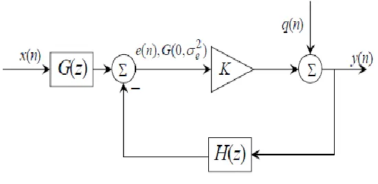
[image:3.612.170.445.157.291.2]A quasi-linear model of a Δ-Σ modulator is shown in Fig.1, where G(z) is the input transfer function, H(z) the feedback filter transfer function and the quantizer is replaced by a gain factor K followed by an additive white quantization noise source q(n):
Fig. 1. Quasi-linear Δ-Σ modulator.
Assuming q(n) to be white with zero mean and variance σq2, and the Noise Transfer Function (NTF) between q(n) and y(n) to be known, the noise variance V0 at the output of the Δ-Σ modulator is given by [10]:
1
0
2 2
2
K A df e NTF
Vo q jf q (1)
where, A(K) is the Noise Amplification Factor. Using Parseval’s theorem, A(K) can also be found in the time-domain as [10]:
2 2 20
ntf n
ntf K
A
n
(2)
where ntf(n)is the impulse response corresponding to NTF(z) and ||ntf||2 2
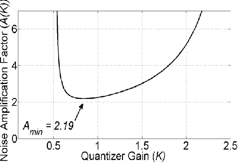
Fig. 2. Noise Amplification Factor variation with quantizer gain.
The Δ-Σ modulator is considered to be stable in the positive slope section of the A(K) curve. If K increases slightly in this section, A(K) increases which results in more circulating noise which in turn tends to decrease K; the system is therefore in equilibrium. As the input amplitude increases A(K) continues to decrease thereby reaching a point when A(K) reaches Amin, where the Δ-Σ modulator commences to operate in the negative slope region in which there is no equilibrium and hence becomes unstable. For stable operation of the Δ-Σ modulator therefore, A(K) > Amin.[10]. If one can quantify the variation of A(K) with the input signal amplitude a for which A(K)> Amin, then the maximum stable input amplitude limits can be established. Quantifying A(K) is done in two steps, first by estimating the ratio of signal variance to quantization noise variance at the input to the quantizer gain K and subsequently estimating the variation of quantization noise variance σq2 with the input signal amplitude in the Δ-Σ modulator loop.
III. SIGNAL AND NOISE VARIANCE AT QUANTIZER INPUT AND QUANTIZATION NOISE
A. The ratio of the signal variance to quantization noise variance at the quantizer input.
Consider an input signal, consisting of five incommensurate sinusoids with the variances σi 2
5 1 2 2 i i x
(3)
If σex2 and σeq2 are variances of the signal and quantization noise at the input to the quantizer, as the signal and quantization noise are uncorrelated the combined variance at the quantizer input is given by:
e2 ex2 eq2 (4)
The quantizer gain K of a Δ-Σ modulator for a Gaussian input with variance σe2 for a single-bit output is given by [26]:
2 e
K (5)
Defining ρ2 as the ratio of the signal variance to the quantization noise variance at the quantizer input yields the equation below:
2 2 2 eq ex
(6)
The quantizer gain K can be found from (4), (5) and (6) as given by:
2 1 1 2 eq
K (7)
The Signal Transfer Function (STF) of the Δ-Σ modulator should ideally be ≈ 1, therefore:
K2ex2 2x (8)
From (3) the variance of the signal consisting of five sinusoids each with equal amplitudes is given by:
5 2 1 2 2 2 5 2 1 i i i
x a a
(9)
As ∆ can be assumed to be equal to 1 for a single-bit quantizer, one gets the following relation from (7), (8) and (9):
2 2 2 2 2 2 5 ] 1 [ 1 2 i x eq
ex a
(10)
2 2 2 2 5 ] 1 [ 1 2 i a
(11)
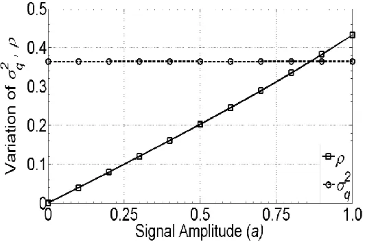
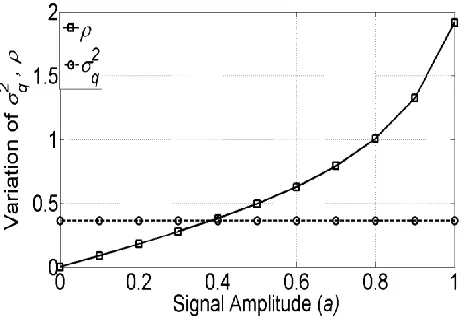
By solving (11), we get ρ which is plotted in Fig. 3. The variation of ρ is plotted as a function of amplitude a such that
5 1 i ia
a
. This has been done to facilitate the comparative analysis with that of a single-sinusoidal input with amplitude a. It isFig. 3. Variation of σq2 and ρ.
B. Quantization noise variance.
If E(.) is the expectation operator, the power at the output of the Δ-Σ modulator is given by:
E[y2
n]q2K2ex2 K2eq2 2 (12)The quantization noise variance σq2 can be found from (7), (8) and (12):
] 1 [ 1 2 ] 1 [ 2 1 2 2 2 2 2
q (13)
Assuming ∆ as ±1 for the single-bit quantizer, the quantization noise variance σq2 is obtained from (13) and is plotted as in Fig. 3. The quantization noise variance remains constant as the signal amplitude increases.
C. Noise Amplification Factor.
Thenoise variance at the output of a Δ-Σ modulator is:
Vo q2 K2eq2 (14) From (7) and (14) we get:
2 2 1 1 2 q o
V (15)
2 2 2 2 1 1 2 ) ( q q q o V K A
(16)
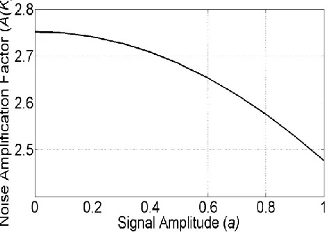
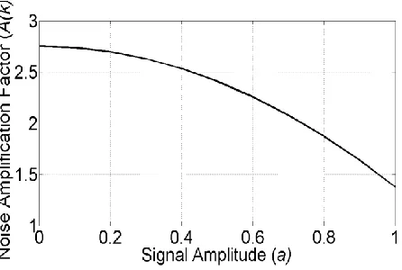
[image:7.612.182.419.261.428.2]Using (16), A(K) is plotted in Fig. 4. It decreases as the sum of sinusoids a increases reaching Amin at which point the Δ-Σ modulator becomes unstable. From (1) and (16), it is seen that as the Δ-Σ modulator order increases, so does Vo thereby increasing A(K) in Fig. 2. Thus, the Δ-Σ modulator gets unstable at lower amplitudes for a higher NTF order. On the other hand, as the number of quantizer bits increases, the quantization noise σq2 decreases, thereby lowering A(K) and Aminand increasing the input stable amplitude limit for the same NTF order.
Fig. 4. Variation of A(K ) with signal input amplitude for multiple-sinusoids
D. Comparison with a single-sinusoidal input.
For a single-sinusoidal input with amplitude a the signal variance γ2 is given by:
2 2
2 1
a
(17)
From (11) one can get an equivalent relation:
2 2 2 2 1 ] 1 [ 2 a
(18)
Fig. 5. Variation of σq2 and ρ for single-sinusoidal input.
The ρ values obtained for the single-sinusoid input are higher than those for the multiple-sinusoidal inputs. This is because the signal variance at the input to the quantizer is higher for the single-sinusoidal with an amplitude a than for a multiple-sinusoid of
equal amplitudes ai such that
51 i
i
a
a
.This is illustrated by the variation of σq2 and γ2 with ai for i=5 in Fig.6. [image:8.612.46.546.291.564.2]
Fig. 6. Variation of σx2 and γ2 with ai.
Fig. 7. Variation of A(K ) with signal amplitude for single-sinusoidal.
E. Multi-bit quantizer-present approach limitation.
This section concerns the limitations that are associated with the current approach for the multi-bit quantizer case. The concept of modified non-linearity can be used to find the mid-rise and mid-thread multi-bit quantizer gains from first principles and are given in [26]. Consider a simple case of a 3-level mid-thread multi-bit quantizer with the parameter δ , the point at which the quantizer step rises as shown in Figure 8.
Fig. 8. 3-level multi-bit quantizer.
The multi-bit quantizer gain Km for a mid-thread quantizer is given by [26]:
e e
m PF
K
2 (19) where,
2
2
2 1 ) (
x
e x
PF
(20) Assuming a uniform quantizer we have:
2
Using equations (19), (20) and (21) the multi-bit quantizer gain is given by:
2 e m
K (22)
where
2
2
8 e
e
(23)
Comparing (22) and (5), we observe that the multi-bit quantizer has an additional exponential term as a function of the input variance e
2
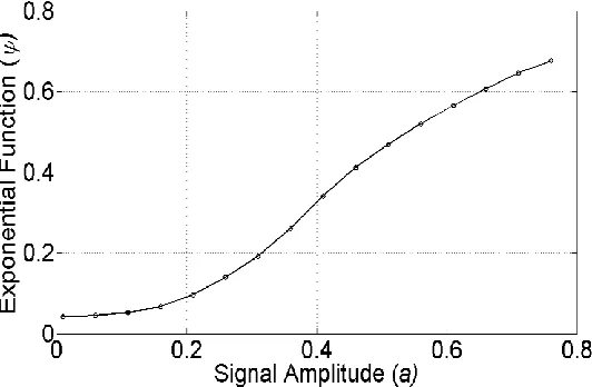
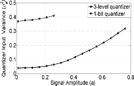
as compared to the single-bit quantizer. It is therefore very mathematically challenging to split the variance of the signal and quantization noise at the input to the quantizer as done in the single-bit case using (6) and continue with similar analysis as before. One possible approach may be to model the exponential function as another function that may permit separation of the variances which would enable one to proceed with the analysis as has been done for the 1-bit quantizer using (7)-(16). Using (23), the variation in ψ for the 3-level uniform quantizer shown in Fig. 8 with Δ = ± 1 for a 5th-order Δ-Σ modulator is shown in Fig. 9. The variation does offer some insight into the stable nature of the 3-level quantizer. As ψ reduces the 3-level quantizer gain value Km by almost a factor of 1/10 for a = 0.1 as compared to K , this along with the fact that the quantization noise variance is less for the 3-level quantizer as compared to the 1-bit quantizer, the variance at the quantizer input e2 is lower for the 3-level quantizer as compared to the 1-bit quantizer for the same input single amplitude a.For a 5th -order Δ-Σ modulator, this is shown in Figure 10 wherein the 3-level quantizer gets unstable at a = 0.75 where e
2
= 0.34. The 1-bit quantizer has a comparable e2 = 0.41 for a much lower value of a = 0.24, at which point the Δ-Σ modulator gets unstable. Further work, however, would be required for a comprehensive explanation for the stability analysis of multi-bit quantizers based on the concept given in sections III A-D.
[image:10.612.169.435.533.707.2]Fig. 10. Variation of quantizer input variance with signal amplitude.
IV. SIMULATION RESULTS
A. Simulation Results.
[image:11.612.168.428.58.225.2]Simulations were undertaken for 3rd-, 4th- and 5th-order single-loop single-bit Δ-Σ modulators. The corresponding A(K) curves for these Δ-Σ modulators are shown in Fig 11.. The Amin values for the curves are 2.11, 2.41 and 2.67 respectively.
Fig.11. Variation of Noise Amplification Factor with quantizer gain.
The Δ-Σ modulators were implemented by deploying a cascade-of-accumulators feedback-form (CAFB) topology as shown in Fig. 12. for the 4th-order Δ-Σ modulator case.
[image:11.612.184.427.441.603.2]Fig.12. Fourth-order Δ-Σ modulator in CAFB topology.
The coefficient values for the three Δ-Σ modulators are shown in Table I.
TABLEI
COEFFICIENTS FOR Δ-ΣMODULATORS
Δ Σ i 1 2 3 4 5 6
5th-order
δi 0.0028 0.0334 0.1852 0.5904 1.1120 1.0000
αi 0.0028 0.0334 0.1852 0.5904 1.1120 -
βi 1.0000 1.0000 1.0000 1.0000 1.0000 -
γi 0.0007 0.002 - - - -
4th-order
δi 0.0157 0.1359 0.5140 0.3609 1.0000 -
αi 0.0157 0.1359 0.5140 0.3609 - -
βi 1.0000 1.0000 1.0000 1.0000 - -
γi 0.003 0.0018 - - - -
3rd-order
δi 0.0751 0.0421 0.9811 1.0000 - -
αi 0.0751 0.0421 0.9811 - - -
βi 1.0000 1.0000 1.0000 - - -
γi 0.0014 - - - - -
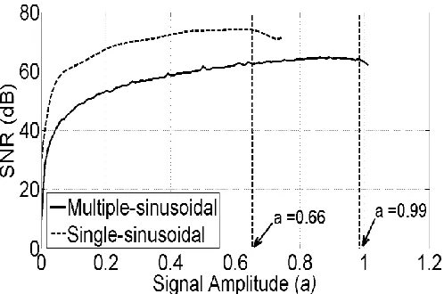
Fig. 13. 3rd-order variation of SNR with input signal amplitude.
[image:13.612.174.424.516.696.2]The SNR increases linearly with an increase in a. The SNR for the single-sinusoidal input remains higher than the multiple- sinusoidal input due to the greater signal variance. As the variance of the signal at the quantizer input is also higher, the Δ-Σ modulator becomes unstable at the lower value of a= 0.66 than it does for the multiple-sinusoidal input for a = 0.99. At a = 0.66, it starts to fall showing the onset of instability for the single-sinusoidal input. The numerical stable value of a as predicted from Fig. 7 is 0.68, when A (K) = 2.11 = Amin. The predicted stable value of 0.68 is very close to 0.66 that is obtained via simulations. The SNR for the multiple-sinusoidal input falls at a = 0.99 indicating the onset of instability.The numerical stable value of a as predicted from Fig. 4 is 1.55 when A (K) = 2.11. The variation in the SNR with a for the 4th-order Δ-Σ modulator is shown in Fig. 14.
The 4th-order Δ-Σ modulator is stable up to a = 0.47 for the single-sinusoidal input. The numerical stable value of a as predicted from Fig. 7 is 0.49, when A (K) = 2.41 = Amin. For the multiple-sinusoidal case, the SNR starts to fall at a = 0.61, at which point the Δ-Σ modulator becomes unstable. The numerical stable value of a as predicted from Fig. 4 is 1.3, when A (K) = 2.41 = Amin. The variation in the SNR with a for the 5th-order Δ-Σ modulator is shown in Fig. 14.
Fig. 15. 5th-order variation of SNR with input signal amplitude.
At a = 0.21, it starts to fall showing the onset of instability for the single-sinusoidal input. The numerical stable value of a as predicted from Fig. 7 is 0.23, when A (K) = 2.67 = Amin. For the multiple-sinusoidal input, the stable amplitude limit is 0.37. The numerical stable value of a from Fig. 4 is 0.38, for Amin = 2.67. The gain in the SNR is 5 dB as a increases from the stable input amplitude limit of 0.21 for the single-sinusoidal input to the 0.37 input amplitude limit for the multiple-sinusoidal input.
B. Accuracy of Results.
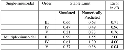
The numerically predicted stable amplitude limits along with the ones obtained via simulations are shown in Table II.
TABLEII
SIMULATION VALUES
Single-sinusoidal Order Stable Limit Error
in dB Simulated Numerically
Predicted
III 0.66 0.68 0.71
IV 0.47 0.49 0.96
V 0.21 0.23 0.76
Multiple-sinusoidal III 0.99 1.55 2.00
IV 0.61 1.30 4.00
[image:14.612.183.432.617.716.2]It is observed that the predicted values from the A (K) curves are more accurate for the single-sinusoidal input as compared to the multiple-sinusoidal input for the 3rd- and 4th-order cases. In addition the numerically predicted values for the single-sinusoidal input are more accurate with this simpler approach with a single quantizer gain in comparison to employing separate signal and noise gains as in [11]-[14]. Accurate results can be predicted for the 5th-order for both the single- and multiple-sinusoidal inputs. This can be attributed to the validity of the assumption that the input at the quantizer input has a Gaussian PDF. This assumption must hold for the quantizer gain given by (5) on which the analysis is based. The input to the quantizer, which is a combination of the quantization noise with a Uniform PDF and the signal PDF, tends to be less Gaussian for the multiple-sinusoidal input as compared to the single-sinusoidal input that tends to be more Gaussian, hence leading to more accurate results in the latter case. The is established by undertaking the Kolmogorov-Smirnov (KS) Gaussian test, according to which the test static (ks)is given by [27]:
ks max
F
x G x
(16) where F(x) is the cumulative density function (CDF) of the quantizer input and G(x) is the standard Gaussian CDF used for this test, the lower the value of ksthe closer is the quantizer input to having a Gaussian PDF. The variation of ks values for the 3rd-, 4th- and 5th-order Δ-Σ modulator quantizer inputs with the signal amplitude a are shown in Fig.16, 17 and 18 respectively. For the 3rd- and 4th- order Δ-Σ modulators, it is observed that the single-sinusoidal input has lower ks values as compared to the multiple-sinusoidal input indicating a more Gaussian PDF. For the 5th-order Δ-Σ modulator in Fig 18, the ks values are almost the same and lower than those for the 3rd- and 4th- order Δ-Σ modulators. [image:15.612.172.422.526.693.2]This validates the assumption that the input to the quantizer, when it undergoes a triple- or higher-order integration tends to make the input a Gaussian distribution. More accurate results, therefore, are predicted in Table II for the 5th-order Δ-Σ modulator for the multiple-sinusoid input than for the 3rd- and 4th-order Δ-Σ modulator.
Fig. 16. 3rd-order variation of k
Fig. 17. 4th-order variation of k
s with input signal amplitude.
Fig. 18. 5th-order variation of k
s with input signal amplitude.
For any NTF, one can plot the A(K) curve and accurately predict stability of the Δ-Σ modulator from Fig. 4 and Fig. 7 circumventing the need for elaborate and time consuming detailed simulations.
V. CONCLUSIONS
[image:16.612.173.426.306.481.2]number of sinusoids greater than five, for any NTF, be it low-pass or band-pass or any other. The Δ-Σ modulator relationship between stability, increase in the NTF order and the number of quantizer bits has been mathematically explained and novel results are reported. The novel results would enable optimizing the design of higher-order Δ-Σ modulators for various applications that require multiple-sinusoidal inputs such as speech processing and moreover for any general inputs that can be modeled as the Fourier series decomposition of individual sinusoids. The results from this work will also make it possible to design and commission Δ-Σ modulators for the applications mentioned without the need for exhaustive time consuming stability analysis and simulations. The analysis, although becomes more complicated can be extended to multi-level quantizers, the results of which would be reported in a future publication.
REFERENCES
[1] Hein, S., and Zakhor, A.: ‘On the stability of sigma-delta modulators’, IEEE Trans. on Signal Processing, Jul 1993, Vol. 41, No.7, pp. 2322-2348.
[2] Ardalan, S. H., and Paulos, J.J.: ‘An analysis of non-linear behaviour in Σ-Δ modulators’, IEEE Trans. on Circuits and Systems, Jun 1987, Vol. CAS-34, No. 6, pp. 1157-1162.
[3] Steiner, P., and Yang, W.: ‘Stability analysis of the second-order sigma-delta modulator’. Proc. IEEE Int. Sym. on Circuits and Systems-ISCAS 94, 1994, Vol. 5, pp. 365-368.
[4] Fraser, N. A., and Nowrouzian, B.: ‘A novel technique to estimate the statistical properties of sigma-delta A/D converters for the investigation of DC stability’. Proc. IEEE Int. Symp. on Circuits and Systems-ISCAS 02, May 2002, Vol.3, pp.111-289-111-292.
[5] Wong, N., and Tung-Sang, N.G.: ‘DC stability analysis of higher-order, lowpass sigma-delta modulators with distinct unit circle NTF zeroes’, IEEE Trans. on Circuits & Systems-II: Analog and DSP, Vol. 50, Issue 1, Jan 2003, pp. 12-30.
[6] Zhang, J., Brennan, P.V., Juang, D., Vinogradova, E., and Smith, P.D.: ‘Stable boundaries of a 2nd-order sigma-delta modulator’. Proc. South. Symp. on Mixed Signal Design, Feb 2003, pp. Feb 2003.
[7] Zhang, J., Brennan, P.V., Juang, D., Vinogradova, E., and Smith, P.D.: ‘Stable analysis of a sigma-delta modulator’. Proc. IEEE Int. Symp. on Circuits and Systems-ISCAS 03, May 2003, Vol.1, pp.1-961-1-964.
[8] Reiss, J.: ‘Stability analysis of limit cycles of higher-order sigma-delta modulators’. 115th Audio Engineering Society (AES) Convention, Oct 2003, New York, USA.
[9] Reiss, J.: ‘Towards a procedure for stability analysis of higher-order sigma-delta modulators’. 119th Audio Engineering Society (AES) Convention, Oct 2005, New York, USA.
[10] Risbo, L.: ‘Stability predictions of higher-order delta-sigma modulators based on quasi-linear modeling’. Proc. IEEE Int. Symp. on Circuits and Systems-ISCAS 94, 30 May-02 Jun 1994, Vol.5, pp. 361-364.
[11] Lota, J., Al-Janabi, M., and Kale, I.: ‘Stability analyses of higher-order delta-sigma modulators using the Describing Function method’. Proc. IEEE Int. Symp. on Circuits and Systems-ISCAS 2006, May 2006, pp. 593-596.
[12] Lota, J., Al-Janabi, M., and Kale, I.: ‘Stability analyses of higher-order delta-sigma modulators for dual-sinusoidal inputs’. Proc. IEEE Inst. and Measurements Technology Conf.-IMTC 2007, Warsaw, Poland, pp. 1-5.
[13] Lota, J., Al-Janabi, M., and Kale, I.: ‘Nonlinear stability analyses of higher-order sigma-delta modulators for DC and sinusoidal inputs’, IEEE Trans. on Inst. and Measurements, Mar 2008, Vol. 57, No. 3, pp. 530-542.
[14] Altinok, D.G., Al-Janabi, M., and Kale, I.: ‘Stability analysis of bandpass sigma-delta modulators for single- and dual-tone sinusoidal input’, IEEE Trans. on Inst. and Measurements, Feb 2011, Vol. PP, Issue 99, pp. 1-9.
[15] Rebai, C., Ghazel, A., and Farhat, F. : ‘High order 1-bit sigma-delta ADC for multistandard GSM/UMTS radio receiver’. Proc. 16th Int. Conf. on Microelectronics, ICM 2004, Dec 2004, pp. 128-131.
[17] Kuei-Chih, Lin., Chuan-His, Liu.: ‘On the design and analysis of the 4th-order leapfrog sigma-delta modulator’. Proc. Int. Conf. on Comm, Ckts and Syst, ICCCAS-2006, Jun 2006, Vol. 4, pp. 2304-2308.
[18] Youngkil, Choi., Hyungdong, Roh., Hyunseok, Nam., and Jeongjin, Roh..: ‘99-dB High-Performance Delta-Sigma Modulator for 20-kHz Bandwidth’. Proc. 4th IEEE International Symposium on Electronic Design, Test and Applications, Jan 2008. DELTA 2008, pp.75-78.
[19] Jeongjin, Roh., Sanho, Byun., Youngkil, Choi., Hyungdong, Roh., Yi-Gyeong, Kim., Jong-Kee, Kwon.: ‘A 0.9-V 60-μW 1-bit fourth-order delta-sigma modulator with 83-dB dynamic dange’, IEEE Journal of Solid-State Circuits, Feb 2008, Vol. 43, pp. 361-370.
[20] Eid, E.-S. and Gaber, W.M. : ‘Design of a 0.9-V 5-MHz sampling frequency 120-µW 1-bit fourth-order feedforward Sigma-Delta modulator’, Proc. IEEE TENCON 2009, Jan 2009, pp.1-4.
[21] Youngkil, Choi., Jeongjin, Roh., Hyungdong, Roh., Hyunseok, Nam., and Songjun, Lee.: ‘A 99-dB DR fourth-order delta–sigma modulator for 20-kHz bandwidth sensor applications’, IEEE Trans. on Inst. and Measurements, Jul 2009, Vol. 58, Issue 7, pp. 2264-2274.
[22] Yang, Zhenglin., Yao, Libin., and Lian, Yong.: ‘A 0.7-V 100-µW audio delta-sigma modulator with 92-dB DR in 0.13-µm CMOS’. Proc. IEEE Int. Sym. on Ckt. and Sys., ISCAS 2011, May 2011, pp. 2011-2014.
[23] Liyuan, Liu., Run, Chen., and Dongmei, Li.: ‘A 20-Bit Sigma-Delta D/A for Audio Applications in 0.13um CMOS’. Proc. IEEE Int. Sym. on Circuits and Systems-ISCAS 2007, May 2007, pp. 3622-3625.
[24] Analog Devices.: ‘Omni-directional microphone with bottom port and digital output’, Data Sheet for ADMP 421. Available at:
http://www.analog.com/static/imported-files/data_sheets/ADMP421.pdf, accessed on Oct 2011.
[25] Fang, W., and Toth, Mark.: ‘Using the digital microphone function on TLV320AIC33 with AIC33EVM/USB-MODEVM system’. Texas
Instruments Application Report SLAA275, Nov 2005. Available at: http://www.ti.com/lit/an/slaa275/slaa275.pdf, accessed on Oct 2011. [26] Gelb, A., and Velde, W. E. V.: ‘Multiple-Input Describing Functions and Nonlinear System Design’ (McGraw-Hill Book Company), Appendix E
Table of Random-Input Describing Functions (RIDFs), pp. 565-588.