Published by Faculty of Science, Kaduna State University.
Algorithm for Solving a Generalized Hirota-Satsuma Coupled KDV Equation Using Homotopy Perturbation Transform Method
ALGORITHM FOR SOLVING A GENERALIZED HIROTA-SATSUMA
COUPLED KDV EQUATION USING HOMOTOPY PERTURBATION
TRANSFORM METHOD
1Lawal, O. W., 2Loyimi, A.C. and 2Erinle-Ibrahim, L. M. 1Department of Mathematics, University the Gambia, Gambia
2Department of Mathematics, Tai Solarin University of Education, Ijagun, Ogun State
*Corresponding Author’s Email Address: [email protected]
ABSTRACT
In this paper, we merge homotopy perturbation method with He’s polynomials and Laplace transformation method to produce a highly effective algorithm for finding approximate solutions for generalized Hirota-Satsuma Coupled KdV equations. This technique is called the Homotopy Perturbation Transform Method (HPTM). With this technique, the solutions are obtained without any discretization or restrictive assumptions, and devoid of round-off errors. This technique solved a generalized Hirota-Satsuma Coupled KdV equation without using Adomian’s polynomials which can be considered as a clear advantage over the decomposition method. MAPLE software was used to calculate the series generated from the algorithm. The results reveal that the homotopy perturbation transform method (HPTM) is very efficient, simple and can be applied to other nonlinear problems.
Keywords: Coupled KdV equations, Homotopy perturbation transform method, Laplace transform method, Maple software, He’s polynomial
INTRODUCTION
The Korteweg-de Vries equation is a mathematical model of waves on shallow water surfaces. It is mostly notable as the prototypical example of a differential equation whose solution can be precisely specified.
The Coupled Kortweg-de Vries (Ckdv) equation describes interaction of two long waves with different dispersion relations. It is connected with most types of long waves with weak dispersion, internal acoustic and planetary waves in geophysical hydrodynamics. The CKdv equation has several connections to physical problems. It approximately describes the evolution of long, one dimensional waves in many physical settings such as ion acoustic waves in a plasma, shallow-water waves with weakly non-linear restoring forces, long internal waves in a density-stratified ocean and acoustic waves on a crystal lattice.
Here, we consider a generalized Hirota-Satsuma coupled KdV equation which was one of the equations introduced by Wu et al. (1999). They introduced a
4
4
matrix spectral problem with three potentials and proposed a corresponding hierarchy of nonlinear equations; one of the typical equations in hierarchy is generalized Hirota-Satsuma coupled KdV equation.x
uw
x
u
u
x
u
t
u
(
)
3
3
2
1
3 3
(1)
x
v
u
x
v
t
v
3
3 3(2)
x
w
u
x
w
t
w
3
3 3(3)
Equations (1) - (3) above are reduced, respectively, to a new complex coupled KdV Equation (Wu et al., 1999) and Hirota-Satsuma Equation (Hirota & Hirota-Satsuma, 1981)
Several methods have been used recently for solving equations (1) - (3) simultaneously with different solutions presented as well. Recently, Dalal (2012) considered the homotopy perturbation method (HPM) to obtain the exact solution of Hirota-Satsuma Coupled KdV equation using MATLAB. Some other authors that solved equations (1) – (3) include, Jacobi elliptic function method by Yu et al. (2005), the projective Riccati equations method by Yong et al. (2005), the algebraic method by Zayed et al. (2004), Adomian’s decomposition method by Kaya (2004), homotopy perturbation method by Ganji & Rafei (2006), variational iteration method by He & Wu (2006) and Assas (2008), homotopy analysis method by Abbasbandy (2007), homogenous balance method by Yong et al. (2003), differential transform method by Figen & Fatma (2010), the trigonometric function transform method by Cao et al. (2002) and Jacobian and rational methods by Zayed et al. (2007).
He (2003) developed the homotopy perturbation method (HPM) by merging the standard homotopy and perturbation for solving various physical problems. HPM can be applied to linear and nonlinear problems without any discretization, restrictive assumption or transformation and is free from round off errors. The Laplace transform cannot handle nonlinear equations because of the difficulties that are caused by the nonlinear terms. Various ways have been proposed recently to deal with these nonlinearities such as the Adomian decomposition method (Biazar et al., 2010) and the Laplace decomposition algorithm (Khuri, 2001; Yusufoglu, 2006; Islam et al., 2010).
Here, the homotopy perturbation method was combined with the He’s polynomials and well-known Laplace transformation method (Madan & Fathizadeh, 2010) to produce a highly effective algorithm and technique for handling a generalized Hirota-Satsuma Coupled KdV equation. This technique called homotopy perturbation transform method (HPTM) provides the solution in a rapid convergent series which may lead to the solution in a closed form. The advantage of this method is its capability of combining two powerful methods for obtaining exact solutions for
Hirota-Fu
ll L
en
gt
h Rese
ar
ch
Algorithm for Solving a Generalized Hirota-Satsuma Coupled KDV Equation Using Homotopy Perturbation Transform Method
Satsuma Coupled KdV equations.
Moreover, contrary to the conservative methods which require the initial and boundary conditions, the HPTM provide an exact solution by using only the initial conditions. The boundary conditions can be used only to justify the obtained result. A comparison will be made to show that the method is equally able to arrive at exact solutions of Hirota-Satsuma Coupled KdV equations obtained in Dalal (2012).
HOMOTOPY PERTURBATION TRANSFORM METHOD (HPTM)
To illustrate the basic concept of HPTM, we consider a general nonlinear partial differential equation. This is given as introduced by Khan & Wu (2011) by combining the HPM and the LTM for solving various types of linear and nonlinear partial differential equations. Consider the general equations with the initial conditions given by
)
,
(
)
,
(
)
,
(
)
,
(
x
t
Ru
x
t
Nu
x
t
g
x
t
Du
(4))
(
)
0
,
(
x
h
x
u
,u
(
x
,
t
)
f
(
x
)
(5)where D is the nth order ordinary differential and n
n
dx
d
D
.R
is the linear differential operator of less order than D. N represents the general non-linear differential operator andg
(
x
,
t
)
is the source term.Taking the Laplace transform (denoted in the paper by
L
) on both sides of the equation (4)
( , )
( , )
( , )
( , )
L Du x t
L Ru x t
L Nu x t
L g x t
(6)
2 2 2 2
( , )
( ) ( ) 1 1 1
( , ) ( , ) ( , )
L u x t
h x f x
L Ru x t L g x t L Nu x t
s s s s s
(7)
Operating with the Laplace inverse on both sides of (7) gives
1 2
1
( , ) ( , ) ( , ) ( , )
u x t G x t L L Ru x t Nu x t
s
(8)where
G
(
x
.
t
)
represents the term arising from the source term and the prescribed initial conditions.Now, we apply the homotopy perturbation method;
)
,
(
)
,
(
0
t
x
u
p
t
x
u
nn n
(9) And the nonlinear term can be decomposed as
)
(
)
,
(
0
u
H
p
t
x
Nu
nn n
(10) For some He’s polynomial
H
n(
u
)
(Madani & Fathizadeh, 2010) that are given by;0 1
0 0
( , ,...,
)
1
,
0,1, 2,...
!
n n
n
i i n
i p
H u u
u
d
N
p u
n
n dp
(11)
Substituting (9) - (11) in Eq. (8), we get
1 2
0 0
0
1
( , ) ( , ) ( )
( . )
n n
n n
n n
n n n
G x t p L L R p u x t N p H u
s
p u x t
(12)which is the coupling of the Laplace transform and the homotopy perturbation method using He’s polynomials. Comparing the coefficients of like powers of
p
, the following are obtained:0 0
:
( , )
( , )
p
u x t
G x t
(13)
1
1 2 0 0
1
:
( , )
( , )
( )
p
u x t
L Ru x t
H u
s
(14)
2
2 2 1 1
1
:
( , )
( , )
( )
p
u x t
L Ru x t
H u
s
(15)
3
3 2 2 2
1
:
( , )
( , )
( )
p
u x t
L Ru x t
H u
s
(16)
1 1
2
1
:
( )
( , )
( )
n
n n n
p
u x
L Ru
x t
H
u
s
(17)The best approximations for the solutions are
1
0 1 2 3
( , )
( , )
( , )
( , )
( , )
( , )
n n p
u x t
Lim p u x t
u x t
u x t
u x t
u x t
(18)
Experimental Evaluation
To illustrate the basic concepts of HPTM, we consider the system of Equations. (1-3) with the initial conditions as following:
2
3 2
1
( , 0) 2 2 tanh 3
u x k k kx (19)
2 2 2 2
0 2
1 1
4 4
( , 0) tanh
3 3
k c k k k
v x kx
c c
(20)
0 1
( , 0)
tanh
w x
c
c
kx
(21)Taking the Laplace transform on both sides of equations (1) – (3) subject to the initial condition (19) – (21) , we have
3 0
3
( , 0) 1 ( )
( , ) 3 3
2
u x L u L u L vw
L u x t u
s s x s x s x
(22)
0 33
( , 0)
( , )
v x
L
v
3
L
v
L v x t
u
s
s
x
s
x
(23)Algorithm for Solving a Generalized Hirota-Satsuma Coupled KDV Equation Using Homotopy Perturbation Transform Method
0 33
( , 0)
( , )
w x
L
w
3
L
w
L v x t
u
s
s
x
s
x
(24)
The inverse of Laplace transform of equations (22)-(24) implies that 1 3 1 0 3 1 1
1
( , )
( , 0)
2
(
)
3
3
L
L
u
u x t
u x
L
s
s
x
L
u
L
vw
L
u
L
s
x
s
x
(25) 1 0 3 1 1 3( , )
( , 0)
3
L
v x t
v x
s
L
v
L
v
L
L
u
s
x
s
x
(26) 1 0 3 1 1 3( , )
( , 0)
3
L
w x t
w x
s
L
w
L
w
L
L
u
s
x
s
x
(27)Suppose the solution of equations (25)-(27) has the form Let
1
0
( , )
n n( , )
n np
n
u x t
Lim p u x t
p u
(28)1
0
( , )
n n( , )
n np
n
v x t
Lim p v x t
p v
(29)1
0
( , )
n n( , )
n np
n
w x t
Lim p w x t
p w
(30)Now, applying the homotopy perturbation method to equations (25)-(27) and substituting equations
(28)-(30) in to equations (25)-(26)
3
1 1
3
0 0 0
1 0 0 1 0 0 1 3 2 3
( ,0)
n n n n n
n
n n n
n n n n n n n n n u u L L
L p L p u p
s x s x
p
L
L p v p w
s x
L
p u
u x
s
(31) 3 1 1 30 0 0
1 0 0
3
( ,0)
n n n n n
n
n n n
n n n
v v
L L
p L p L p u p
s x s x
L
p v
v x
s
(32)3
1 1
3
0 0 0
1 0 0
3
( ,0)
n n n n n
n
n n n
n n n
w w
L L
p L p L p u p
s x s x
L
p w
w x
s
(33)By expanding equation (31) and comparing the coefficients of like powers of
p
, we have1 0
0 0
:
L
( , 0)
p
u
u x
s
(34)3
1 1 0 1 0
1 3 0
1 0 0
1
:
3
2
6
u
u
L
L
p u
L
L
u
s
x
s
x
w
L
L
v
s
x
(35) 32 1 1 1 1
2 3 0
1 0 1 1
1 0 1 0 1 1 : 3 2 3 6 6 u u L L
p u L L u
s x s x
u w
L L
L u L v
s x s x
w L L v s x (36) 3
3 1 2 1 2 1 1
3 3 0 1
1 0 1 2 1 1
2 0 1
1 0
2
1
: 3 3
2
3 6 6
6
u u u
L L L
p u L L u L u s x s x s x
u w w
L L L
L u L v L v s x s x s x
w L L v s x (37)
31 1 1
3 0 1 0 1 : 3 2 6 k
k k k n
k n n k k n n n u u L L
p u L L u
s x s x
w L L v s x
(38)Expanding equation (32) and comparing the coefficients of like powers of
p
, we have1 0
0 0
:
L
( , 0)
p
v
v x
s
(39)3
1 1 0 1 0
1 3 0
:
L
v
3
L
v
p
v
L
L
u
s
x
s
x
Algorithm for Solving a Generalized Hirota-Satsuma Coupled KDV Equation Using Homotopy Perturbation Transform Method
3
2 1 1 1 1
2 3 0
1 0 1
:
3
3
v
v
L
L
p
v
L
L
u
s
x
s
x
v
L
L
u
s
x
(41) 33 1 2 1 2
3 3 0
1 1 1 0
1 2
: 3
3 3
v v
L L
p v L L u
s x s x
v v
L L
L u L u
s x s x
(42)
31 1 1
3
0
: 3
k
k k k n
k n
n
v v
L L
p v L L u
s x s x
(43)Also expanding equation (33) and comparing the coefficients of like powers of
p
, we have1 0
0 0
:
L
( , 0)
p
w
w x
s
(44)3
1 1 0 1 0
1 3 0
: L w 3 L w
p w L L u
s x s x
(45) 3
2 1 1 1 1
2 3 0
1 0 1 : 3 3 w w L L
p w L L u
s x s x
w L L u s x (46) 3
3 1 2 1 2
3 3 0
1 1 1 0
1 2
: 3
3 3
w w
L L
p w L L u
s x s x
w w
L L
L u L u
s x s x
(47)
3 1 1 3 01
:
k 3 k nn k n k k w L L L L
s s x
w
x
u
p
v
(48)Solving the system of equations (34)-(38) above accordingly with the use of Maple 18.0, we obtain,
3
tanh(
)
1
3
2
3
1
20
k
kx
u
3 2 2
0 1 0
1 1
4tk tanh(kx) 1 2k c ctanh(kx) 2c c
u
(49)
2 6 2 2 6 2
0 0
6 6
3
1 1
2
2 6 2 2
2 6 2 2
0 0
6 6
2
18 sinh( ) tanh( ) 6 sinh( ) tanh( )
1 1 1 1
2 2 2 2
12 sinh( ) tanh( ) 6 sinh( ) tanh( )
3
4 1 1 1 1
2 2 2 2
kx kx kx
kx
kx kx
kx
kx kx
kx kx
t k c kx kx t k c kx kx e c e e c e
e e
t k c kx e kx t k c kx kx
e e
e e
u
2 6 2 2
0 6
2
12 sinh( ) tanh( )
1 1
2 2
kx kx
kx
t k c kx kx e e e (50)
and so on for other components. The solution after third iteration is given by
2 6
2 6 2 2 6 2
0 0
6 6 3
1 1
2
2 0
3 2 2
0 1 0
1
6 3
4
18 sinh( ) tanh( ) 6 sinh( ) tanh( )
1 1 1 1
2 2 2 2
1 2
( , ) 3tanh( ) 1 3 3
4 tanh( ) 1 2 tanh( ) 2
kx kx kx kx
kx kx
n n
t k
t k c kx kx t k c kx kx
e c e e c e
e e
u x t u k kx
tk kx k c c kx c
c
22 6 2 2
2 2
0 0
6 6
2 6 2 2
0 6
2
12 sinh( ) tanh( )
sinh( ) tanh( )
1 1 1 1
2 2 2 2
12 sinh( ) tanh( ) 1 1 2 2 kx kx kx kx kx kx kx kx
t k c kx e kx
c kx kx
e e
e e
t k c kx kx
e e e (51)
Also, solving the system of equations (39)-(43) above accordingly with the use of Maple 18.0, we obtain,
2 2 1 0 0 2 1tanh(
)
4
3
k
k
c
kx
c
v
c
(52)
1 2 3 2 2 3 5 1 ) tanh( 3 4 c k k x k k tv
5 2 1 1 5 22 4 2
2 2 2
2 2
2 2 6
0
2 2
12 1
tanh( ) tanh( ) 1
4
32sinh( ) 12
3 tanh( ) 2
tanh( ) 1
4
3 kx kx
kx kx
kx kx
c c
e e kx kx
k k k
kx k e e kx
kx k c k
e e v t (53)
and so on for other components. The solution after third iteration is given as
5 3 2 2 3 2
2 2 2
1 0
2
0 1 1
2 2
2 2 6
0 5 2 1 1 5 2 2
2 4 2
2 2 2 tanh( ) tanh( ) 4 4 ( , ) 3 3
12 tanh( ) 1 1
4
tanh( ) tanh( ) 1 3
4
32sinh( ) 12 3 tanh( ) 2
n n
kx kx
kx kx
kx kx
t k k x k k k k c kx c
v x t v
c c
kx k c k
c c e e t e e kx kx
k k k
Algorithm for Solving a Generalized Hirota-Satsuma Coupled KDV Equation Using Homotopy Perturbation Transform Method
Solving the system of equations (44)-(48) above accordingly with the use of Maple 18.0, we obtain,
w
0
c
0
c
1tanh(
kx
)
(55)
2 1
1
t
c
k
1
tanh(
kx
)
w
(56)
2
2 6 2 2 2
0 1 5
2
0 2
1 2
4 5 2
4 2
1 2
2 2
1 12 tanh( ) 1 tanh( ) tanh( ) 1
cosh( ) 1 tanh( )
3
tanh( ) 3 tanh( ) 2 4 cosh( ) tanh( ) 1
2 cosh( ) sinh( ) sinh( )
2 cosh ) 3
kx k c kx k c kx
kx kx
c
c kx kx
k kx kx
k kx
c kx
kx
w t
(57)
and so on for other components. The solution after third iteration is given as
2
2 0 2
1 2
4 5 2
1
2
2 6 2 2 2
0 1 5
1 tanh( ) 3
tanh( ) 3 tanh( ) 2
4 cosh( ) tanh( ) 1
2 cosh( ) sinh( ) 2
2
0 1 1
0
1
12 tanh( ) 1 tanh( ) tanh( ) 1
cosh( )
( , ) tanh( ) 1 tanh( )
kx c
t c kx kx
k kx kx
k c kx n
n
kx k c kx k c kx
kx
w x t w c c kx t c k kx
4 2
2
sinh( )
2cosh ) 3
kx
kx
(58)
RESULTS AND DISCUSSION
An approximate solution is obtained of equations (1) - (3) and compared with the exact solution to accentuate the accuracy of the present method. To illustrate the convergence of the HPTM, the results of the numerical example are presented and only few terms are required to obtain accurate solutions. The accuracy of the HPTM for the generalized Hirota-Satsuma Coupled KdV equation is controllable, and absolute errors are very small with the present choice of
t
andx
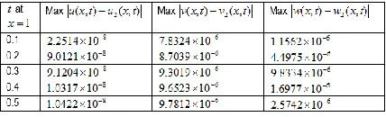
. These results are listed in Tables 1 and 2, it is seen that the method achieves a minimum accuracy of three and maximum accuracy of nine significant figures for equations (1) - (3) for the first two approximations. It is also evident that when more terms for the HPTM are computed the numerical results get much closer to the corresponding exact solutions.Table 1: Maximum pointwise error obtained between HPTM results and exact solutions in Dalal (2012) when
0 1,
c c11,
0.1,
k 1 and
x
0.5
at various value oft
Table 2: Maximum pointwise error obtained between HPTM results and exact solutions in Dalal (2012) when c0 1,c1 1,
0.1,
k 1and x1 at various value of
t
Conclusion
In this research, solutions of Generalized Hirota-Satsuma Coupled KdV equations are obtained by applying homotopy perturbation transform method with specific initial conditions. The results show that the homotopy perturbation transform method (HPTM) is powerful and efficient technique in finding approximate solutions for Generalized Hirota-Satsuma Coupled KdV equations. The numerical results obtain for nth approximation are compared with the known exact solutions and the results show excellent approximation to the actual solutions of the equations by using only three iterations.
It is worth mentioning that HPTM is capable of reducing the volume of the computational work considerably compared to the classical methods while still maintaining the high accuracy of the numerical result; the size reduction amounts to an improvement of the performance of the approach. Hence the method can be considered as a good refinement of existing numerical technique and might find wide application in different fields of science.
REFERENCES
Abbassandy S. (2007). The application of homotopy analysis method to solve a generalized Hirota–Satsuma coupled KdV equation. Phys. Lett. A. 361: 478–483.
Biazar, J., Gholami, M. and Ghanbari, B. (2010), Extracting a general iterative method from an Adomian decomposition method and comparing it to the variational iteration method. Computers & Mathematics with Applications. 59: 622–628. Cao, D. B., Yang, J. R. and Zhang,Y. (2002). Exact solutions for a
new coupled mKdV equations and a coupled KdV equation. Phys. Lett. A. 297: 68–74.
Dalal A. M., (2012). Homotopy Perturbation Method for the Generalized Hirota-Satsuma Coupled KdV Equation. Applied Mathematics. 3: 1983-989
Figen, K. and Fatma, A. (2010). Solitary Wave Solutions For Hirota-Satsuma Coupled Kdv Equation And Coupled Mkdv Equation By Differential Transform Method, The Arabian Journal for Science and Engineering. 35(2), 203–213. Ganji, D. D. and Rafei, M. (2006). Solitary wave solutions for a
generalized Hirota–Satsuma coupled KdV equation by homotopy perturbation method, Phys. Lett. A. 356: 131–137. He, J. H. and Wu, X. H. (2006). Construction of solitary solution
and compacton–like solution by variational iteration method. Chaos, Solitons and Fractals 29(1), 108–113.
He, J.H. (2003). Homotopy perturbation method: a new nonlinear analytical technique. AppliedMathematics and Computation, 135: 73–79.
He, J.H. (2004). Comparison of homotopy perturbation method and homotopy analysis method. Applied Mathematics and Computation. 156: 527–539.
He, J.H. (2004). The homotopy perturbation method for nonlinear oscillators with discontinuities. Applied Mathematics and Computation. 151: 287–292.
He, J.H. (2005). Homotopy perturbation method for bifurcation of
Algorithm for Solving a Generalized Hirota-Satsuma Coupled KDV Equation Using Homotopy Perturbation Transform Method
nonlinear problems, International Journal of Nonlinear Sciences and Numerical Simulation. 6: 207–208.
He, J.H. (2006). Some asymptotic methods for strongly nonlinear equation. International Journal of Modern Physics. 20: 1144–1199.
Hirota, R. and Satsuma, J. (1981). Soliton solutions of a coupled Korteweg–de Vries equation. Phys. Lett. A. 85: 407–408. Islam, S., Faraz, Y. K. and Austin, F. (2010). Numerical solution of
logistic differential equations by using the Laplace decomposition method, World Applied Sciences Journal, 8: 1100–1105.
Kaya, D. (2004). Solitary wave solutions for a generalized Hirota– Satsuma coupled KdV equation. Appl. Math. Comput. 147: 69–78.
Khan, Y. and Wu, Q.(2011). Homotopy perturbation transform method for nonlinear equations using He’s polynomials, Computer and Mathematics with Applications. 61(8) :1963-1967.
Khuri, S.A. (2001). A Laplace decomposition algorithm applied to a class of nonlinear differential equations. Journal of Applied Mathematics. 1: 141–155.
Laila, M. A. (2008), Variational iteration method for solving coupled–KdV equations, Chaos, Solitons and Fractals 38: 1225–1228.
Madani, M. and Fathizadeh, M., (2010). Homotopy perturbation algorithm using Laplace transformation. Nonlinear Science Letters A, 1: 263–267.
Raslan, K. R. (2004). The decomposition method for a Hirota– Satsuma coupled KdV equation and a coupled mKdV equation, Int. J. Comput. Math. 81(12), 1497–1505. Wu, Y. T., Geng, X. G. Hu, X. B. and Zhu, S. M. (1999). A
generalized Hirota–Satsuma coupled Korteweg–de Vries equation and miura transformations. Phys. Lett. A. 255: 259–264.
Yasir K. (2009). An effective modification of the Laplace decomposition method for nonlinear equations. International Journal of Nonlinear Sciences and Numerical Simulation. 10: 1373–1376.
Yasir K. and Naeem F. (2010). A new approach to differential difference equations. Journal of Advanced Research in Differential Equations. 2: 1–12.
Yong, C., Zhen-Ya, Y., Biao, L. and Hong-Qing, Z. (2003). New explicit exact solutions for a generalized Hirota–Satsuma coupled KdV system and a coupled mKdV equation. Chinese Phys. 12(1), 1–10.
Yong, X. L. and Zhang, H. Q. (2005). New exact solutions to the generalized coupled Hirota–Satsuma KdV system. Chaos, Solitons and Fractals. 26(4), 1105–1110.
Yu, Y., Wang, Q and Zhang H. (2005). The extended Jacobi elliptic function method to solve a generalized Hirota– Satsuma coupled KdV equations. Chaos, Solitons and Fractals. 26(5), 1415–1421.
Yusufoglu, E. (2006). Numerical solution of Duffing equation by the Laplace decomposition algorithm. Applied Mathematics and Computation. 177: 572–580.
Zayed, E. M., Zedan, H. and Gepreel, K. A. (2004). On the solitary wave solutions for nonlinear Hirota–Satsuma coupled KdV of equations. Chaos, Solitons and Fractals. 22(2), 285–303.