Numerical Solution of a Free Boundary Problem from Heat Transfer by the Second Kind Chebyshev Wavelets

(1)

Numerical Solution of a Free Boundary Problem from

Heat Transfer by the Second Kind Chebyshev Wavelets

B. Babayar-Razlighi

*

Department of Mathematics, Faculty of Sciences, Qom University of Technology, Qom, Islamic Republic of Iran

Received: 27 April 2019 / Revised: 23 July 2019 / Accepted: 4 September 2019

Abstract

In this paper we reduce a free boundary problem from heat transfer to a weakly

Singular Volterra integral equation of the first kind. Since the first kind integral

equation is ill posed, and an appropriate method for such ill posed problems is based on

wavelets, then we apply the Chebyshev wavelets to solve the integral equation.

Numerical implementation of the method is illustrated by two benchmark problems

originated from heat transfer. The behavior of the initial and free boundary heat

functions along the position axis during the time have been shown through some three

dimensional plots. The convergence of the method is pointed in the end of section 2.

The numerical examples show the accuracy and applicability of the method from

application and programming points of views.

Keywords: Volterra integral equation of the first kind; Heat equation; Numerical solution; Second kind Chebyshev wavelets; Free boundary.

*_{Corresponding author: Tel: +982532941965; Fax: +982536641604; Email: [email protected]} Introduction

In this paper we consider the following free boundary problem from heat transfer in one spatial dimension.

, 0

1,0

,

t xx

u

=

u

< <

x

<

t

(1)

( , 0)

( ), 0

1,

u x

=

f x

< <

x

(2)

( )

0

( , )

( ), 0

(t) 1, 0

,

s t

u x t dx

=

g t

<

s

<

t



(3)

(1, )

( ), 0

.

u

t

=

h t

<

t

(4)

Where

u x t

( , )

is the temperature function and is unknown, and the data and the free boundary function

s(t)

are known.

In [1, 2] the authors have solved similar problems with product integration technique, which is a good method on short time intervals and the second kind integral equations [3-9]. The product integration is not efficient for the integral equations of the first kind.

Since the solution of the associated first kind integral equation is in

L

2

(0,1)

, which is spans by wavelets, hence we solve this problem by wavelets on

[0,1)

. We show the efficiency of the method by two sample problems.

For more application examples of the Chebyshev wavelets for differential and integral equations see [10, 11].

1.Equivalent Integral Equation

(2)

equation is denoted by

2

exp

4

( , )

4

x

t

K x t

t

π



−











=

.

Definition 1.2. The theta function is defined as follow

( , )

(

2 , ),

0.

m

x t

K x

m t

t

θ

∞

=−∞

=



+

>

Proposition 1.3. We have the following list of methods for generating solutions of heat equation from other solutions [12].

Linear combinations: If

u u

₁

,

₂are solutions, then

1 2

u

α

+

β

is a solution, where

α β

,

are constants.

Translations: If

u x t

( , )

is a solution, then so is

(

,

)

u x

−

ξ

t

−

τ

, where

ξ

and _τ are translation parameters.

Convolutions: If

u x t

( , )

is a solution, then so are

(x

, t) ( )

b

a

u

−

ξ φ ξ ξ

d



and

( ,

) ( )

b a

u x t

−

ξ φ ξ ξ

d



.

However

( ,

) ( )

t a

u x t

−

ξ φ ξ ξ

d



is a solution only if

( , 0) 0

u x

=

.

Integrate with Respect to a parameter: If

( , , )

u x t

α

, is a solution for each _α in

a

≤ ≤

α

b

,

then so is

( , , )

b a

u x t

α α

d



.

Affine Transformation: If

u x t

( , )

u x

(

λ λ

,

2

t

)

for any constant

λ

.

Integration with Respect to

x

and

t

: If

u x t

( , )

0

( , )

x

u

ξ

t d

ξ



, provided that

0

( , ) 0.

x

u x t

=

Also, if

u x t

( , )

is a solution, then so

is

( , )

,

t a

u x

η η

d



provided that

u x a

( , ) 0.

=

Lamma 1.4. The bounded solution of

,

0

1, 0

,

( ,0) f( ),

0

1,

(0, t)

(1, t) 0,

0

,

t xx

v

x

t

v x

x

v

t

=

< <

<

=

< <

=

<

is given by

{

}

1

0

( , )

(

, )

(

, ) ( )

.

v x t

=



θ

x

−

ξ

t

−

θ

x

+

ξ

t f

ξ ξ

d

Proof. See exercise 3.6. of [12].

Lamma 1.5. For t >0 ,

1 0

lim 2

( ,

) ( )

0,

t

x

x t

g

d

θ

τ τ τ

− →

∂

−

=

∂



for any Lebesgue integrable g . Moreover, this limit is taken on uniformly with respect to

t

contained in compact sets.

Proof. See lemma 6.2.5 of [12].

Lamma 1.6. For t >0, and piecewise-continuous

,

h

0 1

lim 2

t

(x 1, t

) ( )

( ),

t

x

h

d

h t

θ

τ

τ τ

− →

∂

− −

=

∂



is uniform for

t

belonging to a compact subset of an interval of continuity of

h

.

Proof. See lemma 6.2.3 and last analysis of section 6.2 from [12].

Theorem 1.7. For continuous

f g h

, ,

and

s

with

(0)

0

(0)

( )

s

g

=



f

ξ ξ

d

, the solution of problem (1)-(4)

has the representation

{

}

1 0 0 0

( , ) (x , t) (x , t) ( )

2 (x, t ) ( )

2 (x 1, t ) ( ) , t

t

u x t f d

d x

h d

x

θ

ξ

θ

ξ

ξ ξ

θ

τ φ τ τ

θ

τ

τ τ

= − − +

∂

− −

∂ ∂

+ − −

∂



(5)

if and only if

φ

is a piecewise-continuous solution of the integral equation

{

}

( ) 1 0 0

0 0

( ) (x , t) (x , t) ( ) 2 (0, t ) ( ) 2 ( ( ), t ) ( ) 2 (s(t) 1, t ) ( ) 2 ( 1, t ) ( ) .

s t

t t

g t f d dx

d s t d

h d h d

θ ξ θ ξ ξ ξ

θ τ φ τ τ θ τ φ τ τ

θ τ τ τ θ τ τ τ

− − − +

= − − −

+ − − − − −

 



(6)

Proof. We are going to search

1 2 3

( , )

(3)

1

,

2

u u

and

u

₃satisfy heat equation and each of them meet one of the equations (2)-(4). For this aim let

{

}

1 1

0

2

0

3

0

( , )

(

, )

(

, ) ( )

,

( , )

2

( ,

) ( )

,

( , ) 2

(

1,

) ( ) .

t

u x t

x

t

x

t f

d

u x t

x t

d

x

u x t

x

t

h

d

x

θ

ξ

θ

ξ

ξ ξ

θ

τ φ τ τ

θ

τ τ τ

=

−

+

∂

= −

−

∂

=

−

∂



Let

2

L

t

x

∂

=

−

∂

, by the uniformly convergent of the theta function, _{( , )} _{(x 2 m, t) 0}

m

L x tθ ∞ LK

=−∞

=



+ = .

By the linear combinations and translations of Proposition 1.3,

{ (

θ

x

−

ξ

, )

t

−

θ

(

x

+

ξ

, )} ( )

t f

ξ

is a solution of the heat equation. So according to integrate with respect to a parameter

u x t

₁

( , )

, satisfies the heat equation. From the convolutions of Proposition 1.3, for the investigation of

u x t

₂

( , )

as a solution of heat equation it is sufficient to show that

0

lim

( , ) 0.

t

x

x t

θ

+ →

∂

=

∂

1 0

1

2 3/2 0

2 3/2

0 1

0

2

0

( 2 )

( , ) ( 2 , )

2 lim

( 2 ) ₍ _{2 ,} ₎

2

x exp 2 lim

4

( 2 )

( 2 )exp

2 lim

4

lim ( , )

( 2 )

( 2 )exp 2 lim

m t

m

t

t m t

t

K _{x t} x m _{K x} _{m t}

x t

x m _{K x} _{m t}

t x

t t

x m

t t x t

x

x m

t

τ

π

θ

+

∞ = ∞

→ = → ∞

→ =

→

 

 

 

 

 

 

 

 

 

  =

∂ ₊ − + ₊ ₊

∂

− + ₊ ₋

− −

= +

− + − +

∂ ∂

− − − −

+



3/2 1

0, 4

m

π

t

∞

=



 



 

 ₌



where the uniform convergence of the series allow us to change limit and sigma in lines 4 and 5. Similar

evaluations show that

0

lim

(

1, ) 0

t

x

t

θ

+ →

∂

−

=

∂

, and

hence

u x t

₃

( , )

is a solution of the heat equation.

Substitution of u x t( , )=u x t₁( , )+u x t₂( , )+u x t₃( , ) in (3) and application of Fubini's theorem, forces (6).

Now we investigate the equations (2) and (4).

{

}

1 2 3 1

1 0

0

( , 0) ( , 0) ( , 0) ( , 0) ( , 0)

lim ( , ) ( , ) ( ) (x),

t

u x u x u x u x u x

x t x t f d f

θ

ξ

θ

ξ

ξ ξ

+

→

= + + =

=



− − + =

where the last equality obtained from Lemma 1.4, and hence u satisfies (2). Applications of Lemmas 1.4-1.6 yield that

1 2 3 3

1 0

(1, t)

lim 2

(

1,

) h( )

(t),

t t

u

x

t

d

h

x

θ

τ τ τ

− →

=

+

=

∂

=

−

=

∂



and then u satisfies (4). Since the solution of (1)-(4) is unique (Chapter3 of [12]) then Eq. (5) is the only solution.

2.Chebyshev wavelet technique

Wavelets were first applied in geophysics to analyze data from seismic surveys, which are used in oil and mineral exploration to get "pictures" of layering in the subsurface rock [13]. There are several bases for wavelets, such as Haar wavelet, Daubechies Wavelets, Legendre wavelets, Chebyshev wavelets, and so on [14-17]. In this paper we consider the second kind

Chebyshev wavelets. Chebysheve wavelets

have 4 arguments where

is the order of Chebyshev polynomials and

t

is normalized time. They are defined on the interval

[0,1)

as follow

/2

1 1

,

1

2 2 / (2 2 1)

( ) 2 2

0, .

k k

m k k

n m

n n

U t n t

t

otherwise π

ψ − −

−

 ₋ ₊ _{≤ <}



= 

7)

The coefficient is for the orthonormality, the

dilation parameter is

a

=

2

k−1_{and translation}

parameter is . Here, are the

well- known order second kind Chebyshev polynomials with respect to weight function

2

( )

1

w t

=

−

t

, which is defined on the interval

[ 1,1]

−

. A function

φ

(t)

defined over

[0,1)

can be expressed by the Chebyshev wavelets as

, , 1 0

(t)

n m n m

(t),

n m

c

φ

∞ ∞

ψ

= =

=

 

(8)

where

( )

( , , , )

nm

t

k n m t

ψ

=

ψ

1

1, 2,...., 2 ,

k

,

n

=

−

k

∈

+

m

2

π

(2

1)2

k

b

=

n

−

( )

m

U t

th

(4)

1

, , ,

0

,

(t) (t)

(t) ,

n

n m n m _w n n m

c

=

φ ψ

=



w

φ ψ

dt

(9)

and denotes the inner product in Hilbert space

, and

( )

(

2

k

2

1

)

n

w t

=

w

t

−

n

+

.

One can consider the following truncated approximation for series (8)

1

2 1 , , 1 0

(t)

(t).

k _M

T n m n m

n m

c

C

φ

ψ

− ₋

= =

=

Ψ

 

(10)

Where C and

Ψ

(t)

are vectors, that can be given by

1 1

1,0 1,0

1,1 1,1

1, 1 1, 1

2,0 2,0

2, 1 2, 1

2 ,0 2 ,0

2 , 1 2 , 1 (t) (t)

(t) (t)

; (t) ,

(t)

k k

M M

c c

c c C

c

ψ

− −

 

 

   

= Ψ =

 

(11)

and for the simplicity of numerical evaluations, we rearrange the indices in the second representation of vectors by the mapping

1 1 _{1,i M} 1 ₁ _, _1,...,2k _,

i i _{i i} _M

M M −

    

_ _ _ _ 

_ _ _ _ 

 

− _{+ −} − _{− →} ₌

where [x] denotes the greatest integer less than or equal to x.

The following theorem gives the convergence and accuracy estimation of the second kind Chebyshev wavelets expansion [18].

Theorem 2.1. Let

φ

(t)

be a second-order derivative square-integrable function defined on

[0,1)

with bounded second-order derivative, say

φ

′′

(x) B

≤

for some constant

B

, then

(i)

φ

(t)

can be expanded as an infinite sum of the second kind Chebyshev wavelets and the series converges to

φ

(t)

uniformly, in the form (8).

(ii)

1 , ,

1 2

3 5 4

2 1

0

1 1

0 , ,

2 k (m 1)

k M

m M n

B

as M k n

φ σ

π −

∞ ∞

= = +

≤ ≤

 

→ → ∞

 ₋ 







where

1

2 ₂

1 2 1

, ,

1 0 0

( )

(t) dt

,

k _M

k M nm nm n

n m

t

c

t

w

φ

σ

φ

ψ

− ₋

= =









=



−







 



is the

L

2 norm error.

3.Application of the Method

The integral equation (6) in theorem 2.7 is as follow

0

ker( , ) ( )

( ),

0.

t

τ φ τ τ

d

=

r t t

>



(12)

Where

0

( ) g(t)

_m

(t),

m

r t

∞

r

=

+



(13)

(

)

(

)

( ) 1 0

0 0

0

( ) (x , t) (x , t) ( ) d dx

2

( 1, t

)

(s(t) 1, t

) ( )

,

s t

t

r t K K f

K

h

d

ξ

ξ ξ

τ

τ τ

= − − − +

+

− − −

− −

 



( ) 1

0 0

0

( 1 2 , t ) ( 1 2 , t ) (s(t) 1 2 , t ) (s(t) 1 2 , t )

(x 2 , t) (x 2 , t)

(x 2 , t) (x 2 , t) ( ) d dx

2 ( ) ,

( )

s t

t

m

K m K m

K m K m f

h d

r t m

τ τ

ξ ξ

ξ ξ ξ ξ

τ τ

− + − + − − −

− − + − − − − −

− + + − −

− + + − + −

−

+

= ∈

 

 

 

 

 

 

 



0

ker( , )

ker (t, ),

_m m

t

τ

∞

τ

=



(14)

(

)

0

ker ( , ) 2

t

τ

=

K

(0, t

− −

τ

)

K

(s(t), t

−

τ

) ,

.

2 (2 , t ) ( 2 , t )

(s(t) 2 , t ) (s(t) 2 , t )

( , ) m

K m K m

k er t m

τ τ

τ

− + − −

− + − − − −

= ∈

 

 

 

From the uniform absolute convergence of the series for

θ

( , )

x t

and its partial derivatives, the equation (13) can be approximated by

0 0

( )

( ) ( ) ( ),

( )

N m

m N

T T T

m m

r t

G t R t R t

r t

g t

= =

Ψ + Ψ = Ψ

+



.,.

2

(0,1)

L

1

(5)

where N is sufficiently large positive integer and we apply equation (10) in the second row. Similar evaluations are true for other series of

θ

( , )

x t

and its partial derivatives. Every terms of equations (13) and (14) is evaluable by Mathematica software, and in numerical process the functions in (13) and (14) approximated by some finite terms of sigma, as mentioned for

r(t)

. Using Eq. (10) for approximate

( ) T ( )

φ τ

Φ Ψ

τ

and r(t) _RT_Ψ(t)_{in Eq. (12), forces}

0

(t)

ker( , ) ( )

T

,

0.

t

T

t

τ

τ τ

d

_R

t

Ψ

Φ



Ψ

=

>

(15)

Where ₁ 1

2

,...,

k

T T

M

φ

−

Φ

=









is unknown vector.

Let

0

( )

ker( , ) ( )

t

w t

=



t

τ

Ψ

τ τ

d

, then from Eq. (10)

we obtain

w t

( )

W

Ψ

(t)

, where W is a

1 1

2

k−

M

×

2

k−

M

_{known matrix. Substitution of these} quantities in (13) yields ΦT

W

Ψ =

(t) R

T

Ψ

(t)

. Hence the linear system

W

T

Φ

=

R

, must be solved.

In the following examples we evaluate matrices

,

R W

by the 16-point Gaussian integration rule.

4.Algorithm of the Method

For illustration of superiority and applicability of the method we give an algorithm for the numerical solution of the problem (1)-(4) by the proposed method.

Step1 Input the known functions

f g h s

, , ,

; Define the fundamental solution of heat equation by

2

exp

4

( , )

4

x

t

K x t

t

π



−











=

;

Solve the linear system

W

T

Φ

=

R

as mentioned in section 3 and obtain ( ) T ( )

φ τ

Φ Ψ

τ

. Note that we apply the numerical integration such as Gaussian integration rule for the numerical evaluation of

R

and

W

.

Step2 Since

Ψ

( )

τ

is a piecewise function, then

( )

φ τ

is also a piecewise function. For example with M=5, k=3,

2 3 4

10 11 12 13 14

2 3 4

20 21 22 23 24

2 3 4

30 31 32 33 34

2 3 4

40 41 42 43 44

( )

1 0

4

1 1

4 2

1 3

2 4

3 1 4

0 ,

t

otherwise

φ τ

φ φ τ φ τ φ τ φ τ

 ₊ ₊ ₊ ₊ _{≤ <}

 

 ₊ ₊ ₊ ₊ _{≤ <}

 

 ₊ ₊ ₊ ₊ _{≤ <}

 

 ₊ ₊ ₊ ₊ _{≤ <}

  

which is obtained from step1, and all of

φ

_ij are known constants. The function

u

₂ in the theorem 1.7 is as follow

2

0

2,0 2,m 1

( , )

2

( ,

) ( )

1

( , )

( , ),

2

t

N m

u x t

x t

d

x

u

x t

u

x t

θ

τ φ τ τ

=

∂

= −

−

∂

+





where

2,m

0 2

( 2 , )

( , ) ( ) ,

2

K( 2 , )

t

x m

K x m t

t

u x t d

x m

x m t

t

τ

φ τ τ

τ

+

 

+ − +

 ₋ 

=  

−

 ₋ ₋ 

 

−

 



and

N

is a sufficiently large integer. For evaluation of

2,m

u

, first of all, evaluate on

0

1

4

t

≤ <

, then for

1

4

≤ <

t

2

evaluate 1 4 2,m

0

1 4

2

( 2 , )

( , ) ( )

2

( 2 , )

2

( 2 , )

( ) , 2

( 2 , )

t

x m

K x m t

t

u x t d

x m

K x m t

t

x m

K x m t

t _d

x m

K x m t

t

τ

φ τ τ

τ

φ τ τ

τ

+

 

+ − +

 ₋ 

=  

−

 ₋ ₋ 

 

−

 

+

 

+ − +

 ₋ 

+  

−

 ₋ ₋ 

 

−

 



and so on. Since

φ τ

( )

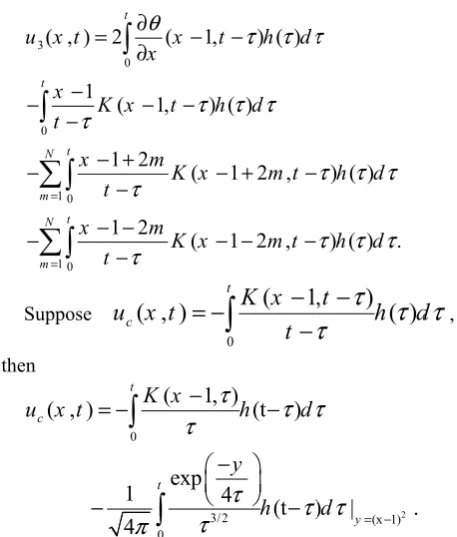
is piecewise polynomial, then these evaluations are straight forward.

(6)

3 0 1 0 1 0 ( , ) 1 t t N m t N m

u x t

x K t x x τ = = = − − − − − − −





Suppose then ( , ) c

u x t =

−

The last in Mathematica

3

( , )

u x t

+

The functi

1( , )

u x t =

where 1,m 1 0

( , )

(

u

x t

K x

ξ

=

−





−

+





are evalua

Step3 Prin where u_j

approximatio integer

N

, e

0

2 ( 1

( 1, )

1 2 ( 1 2 ( t x x

K x t

m K x t m K x t θ τ τ τ ∂ = − ∂ − − − + − − − −



( , )

c

u x t

=

0 0 ( 1 exp 1 4 t t K x

τ

π

− = −    −



ntegral is eval a . Thus we let

1

(x 1) (

(

1

(

1

c N m N m

u x

x

= =

−

+

− +

+

− −



ion

u

₁ in the

{

1 0

1,0

( ,

1 _{( , )} 2

x t

u x t

θ

ξ

= −

+



2 , )

m t

K

m t

ξ

=

+

−

able by any so

nt and plot u(

( , ), j 1, 2x t =

on of u xj( evaluated in st

1, ) ( )

) ( )

1 2 ,

t h d

h d

m t

τ τ τ

τ τ − − + − − − − 0

(

1,

t

K x

t

τ

−



3/2 1, ) (t )

4 _(t ₎

h d

y

h

τ

τ τ

τ

− −      ₋

luable by any t

, )

2 ) (

1

2 ) (

1

c

x t

m u x

−

theorem 1.7 i

1,m 1 ) ( , ( , N m t x

u x t

θ

ξ

= − + +



(

2

(

2

K x

m

K x

ξ

− −

−

+ −

oftware. 1

( , )x t =u x t( , )+ 2,3 are

, )

x t untile su tep 2. ) ( ) ) ( ) . h d h d τ

τ τ τ

,

)

( )

t

h

d

τ τ

τ

−

2 (x 1) )d |_y .

τ

_{= −}

software such

1 2 , )

1 2 , ).

m t

+

−

s

}

) ( ) , ),

t f

ξ ξ

d

, )

( )

2 , )

m t

f

d

m t

ξ







2( , ) 3( u x t u x + +

the trunca ufficiently la

d

τ

,

h as

,

d

ξ

, )t , ated arge 5.N

(

s

is int wit rep sol poi the

(

s

( u T u







F

(

Numerical Ex Example 5

1

3

( )

2

t

=

+

cos f( )x = (x

( , ) e t

u x t ₌ − egral equation th M=5, k=3 presentation fo lution. Table

ints

(0.15i, 0

e three dimens

Example 5

1

2

( )

3

t

=

+

f( ) sin(xx = ( , ) e sin_{x t} ₌ −t

Table 1. The (0.15 i, 0.15

u

9 2.7 10 2.2 1

10 3.1 10 5.2 1

10 3.4 10 3.6 1

10 2.2 10 2.5 1 5.9 − × × − × × − × × − × × ×10 11 1.5 1

11 1.6 10 2.8 1

− _× − × ×





Figure 1. Vari

( , )

x t

for Exam

xamples

.1. In the

,

t

+

g t( ) e= −t ),

x h( ) e c_t ₌ −t cos(x). Wit n (12) by Che , and then w ormula (5) to 1 shows the a

.15 j), ,

i j

=

sional plot of

5.2 In the

,

t

+

g t( )= −e ,

) h( ) e s_t ₌ −t n(x). With

e(i, j)th elem 5 j)−u(0.15

8 9

10 2.4 10

8 8

10 3.7 10

8 9

10 7.6 10

8 8

10 1.2 10

− _× − − _× − − _× − − _× −

8 9

10 1.7 10

8 8

10 1.6 10

− _× − − _× −

ation of the

u

mple 5.1.

e problem

1 1 sin 3 2 t t −    + + (1),

cos The e

th this data, ebyshev wavel we put this so obtain u as absolute error

1,..., 6

. Figu

(x, t)

u



on

[0

problem

e−t_ 1 cos



 _

− +

(1), sin the exa

this data w

ment of the i, 0.15 j) in e

8 3.3 10 5.2 10

8 1.5 10 3.4 10

8 1.9 10 1.7 10

9 5.7 10 1.3 10

− × × − × × − × × − × × 9 4.5 10 2.5 10

8 1.6 10 3.7 10

− × ×

( , )

u x t



as a

(1)-(4), for

, t    exact solution we solve the lets technique olution in the approximated r of u in the ure 1 shows

0,1] [0,1]

×

.

(1)-(4), for

1 1 _,

2 3 t

       + ₊

act solution is we solve the

matrix is example 5.1

9 8

0 1.5 10

8 8

0 2.3 10

8 10

0 9.7 10

8 8

0 1.4 10

− _× − − _× − − _× − − _× −

8 9

0 5.0 10

8 8

0 1.0 10

− _× − − _× −







a function of

(7)

integral equa with M=5, k representatio solution. Sim the absolu

(0.15i, 0.15

three dimens

In this stu following for

( , )

x t

θ

=

+

θ

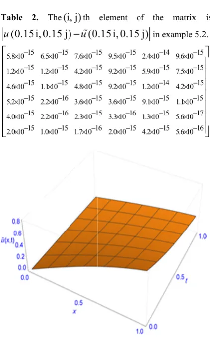
is a un and hence se example see

Table 2. (0.15 i, 0

u

15 5.8 10 6

15 1.2 10 1.

15 4.6 10 1

15 5.2 10 2

− × − × − × − × 15 4.0 10 2

15 2.0 10 1.

− × − ×







Figure 2. V

( , )

x t

for E

ation (12) by C k=3, and then on formula (5) milar to the pre

ute error

5 j), ,

i j

=

1,.

sional plot of

u

R

udy, we consi rm [12]

{

0

( , )

(

m

K x t

K x

∞

=

+



+

niform absolu eries and integ e the corollar

The(i, j)th 0.15 j)−u(0

15 1

.5 10 7.6 10

15 1

.2 10 4.2 10

15 1

.1 10 4.8 10

16 1

.2 10 3.6 10

− − × × − − × × − − × × − − × × 16 1

.2 10 2.3 10

15 1

.0 10 1.7 10

− − × ×

Variation of th Example 5.2

Chebyshev wa n we put this ) to obtain u evious examp

of u in

..., 6

. Figure

(x, t)

u



on

[0

Results

ider the theta

2 , )

m t

K

+

ute convergen gral can be in ry of theorem

element of .15 i, 0.15 j)

15 _{9.5 10}15 _2.4 15 _{9.2 10}15 _5.9 15 _{9.2 10}15 _1.2 15 _{3.6 10}15 _9.

− × × − × × − × × − × 1 15 _{3.3 10}16 _1.3 16 _{2.0 10}15 _4.2

× − × ×

− × ×

he

u x t



( , )

a

avelets techni s solution in as approxima le Table 2 sho

n the po

e 2 shows

0,1] [0,1]

×

.

a function by

(

2 , )

K x

−

m t

nce in its dom nterchanged ( m 7.16 of Ru

the matrix in example 5.2

14 15

10 9.6 10

15 15

10 7.5 10

14 15

10 4.2 10

− − × × − − × × − − × × 15 15

10 1.1 10

15 17

10 5.6 10

15 16

10 5.6 10

− − × × − − × × − − × ×

as a function

ique the ated ows oints the the

}

) .

main for udin [19 rel fre Th the kin suc app of for ben val 1. 2. 3. 4. 5. 6. 7. 8. 9. 10. is 2.







of

9], so we can ations help us ee boundary pr here are many e system of V nd and theta ch problems proaches such wavelets for s r the solution nchmark samp

The author luable suggest

Babayar-Raz an inhomog integration

Mathematics

Babayar-Raz integration m conduction

Mathematics

Orsi A. P. equations of kernels. Math

Criscuolo G Convergence weakly sing 55(191): 213 Babayar-Raz solution for s differential e

Math. Compu

Babayar-Raz solution of n the newton-p

Model. 58: 1 Babayar-Raz Convergence numerical so systems. B. I

Babayar-Raz Badamchizad two- phase s

Soc. 38(4): 8 Babayar-Raz Newton-prod kinetics. J. S

Abd-Elhame New Spect Algorithm f Order Diffe

write the equ s to apply the roblems from heat transfer Volterra integ function repr solved dire h as Runge-Ku

such problem of the system ple problems f

Acknowle

is thankful tions to impro

Refer zlighi B. and Iv geneous heat

method. Th Conference: 5 zlighi B. an method for nu

problem. Th Conference: 86 Product integ f the second

h. Comp. 65(21 G., Mastroia e properties of a gular integral -230 (1990). zlighi B. and S system of singu equations by ne

ut. 219: 8375-8 zlighi B. and S

onlinear singul product integra 696-1703 (2013 zlighi B., Ivaz e of product in olution of line

Iran. Math. Soc

zlighi B., Ivaz deh A., Newto

tefan problem 53-868 (2012). zlighi B., Ivaz duct integration

ci. I. R. Iran. 22 ed W. M., Do ral second k for Solving Lin rential Equatio

uations (13),( proposed me heat transfer problems wh gral equation resentation [1 ectly by som utta methods. ms caused the h m as we have

from heat tran

edgments

to the refere ove this paper

rences vaz K. Numeri

equation by

he 43rd An

15-518 (2012) nd Solaimani umerical solut

he 46rd An

61-864 (2015). gration for Vo

kind with w 15): 1201-1212 anni G. and

a class of produ l equations.

Soltanalizadeh ular nonlinear v newton-product 8383 (2013).

Soltanalizadeh lar volterra inte ation method. M

3).

z K. and Mok ntegration meth

ear weakly sin

c. 37(3): 135-14 z K., Mokhtar

on-product int with kinetics.

.

z K. and Mok n for a stefan 2(1): 51-61 (20 oha E. H. and kind Chebysh inear and nonl

ons Involving

14) and these ethod for such phenomenon. hich reduce to s of the first 12]. Many of me numerical Applicability high accuracy shown in two nsfer.

ees for their .

ical solution of the product

nnual Iranian

.

M. Product ion of a heat

nnual Iranian

olterra integral eakly singular

(1996) . Monegato G. uct formulas for

Math. Comp.

B. Numerical volterra integro-method. Appl.

B. Numerical egral system by

Math. Comput.

khtarzadeh M. hod applied for ngular volterra 48 (2011). zadeh M. and egration for a

B. Iran. Math.

khtarzadeh M. problem with 011).

Youssri Y. H. hev Wavelets linear Second-Singular and

(8)

Bratu Type Equation. Abstr. Appl. Anal. 2013: 9. Article ID 715756 (2013).

11. Biazar J. and Ebrahimi H. Chebyshev wavelets approach for nonlinear systems of volterra integral equations. Comput. Math. Appl. 63: 608–616 (2012)

12. Cannon J. R. The one-dimensional heat equation. Addison-Wesley, Menlo Park, (1984).

13. Boggess A. and Narcowich F. J. A first course in Wavelets with Fourier Analysis. Prentice Hall, (2001). 14. Babolian E. and Shahsavaran A. Numerical solution of

nonlinear Fredholm integral equations of the second kind using Haar wavelets. J. Comput. Appl. Math. 225: 87–95 (2009).

15. Restrepo J.M. and Leaf G.K. Inner product computations

using periodized Daubechies wavelets, Int. J. Num. Methods Eng. 40: 3557–3578 (1997).

16. S. A. Yousefi, Numerical solution of Abel-s integral equation by using legendre wavelets, Appl. Math. Comput. 175(1): 574-580 (2006).

17. Ghasemi M. and Tavassoli Kajani M. Numerical solution of time-varying delay systems by chebyshev wavelets, Appl. Math. Model. 35: 5235–5244 (2011). 18. Zhou F., Xu X., Numerical solution of the convection

diffusion equations by the second kind Chebyshev wavelets. Appl. Math. Comput. 247: 353–367 (2014). 19. Rudin W., Principles of Mathematical Analysis. McGraw