On The Numerical Solution of Urysohn Integral Equation Using Chebyshev Polynomial

International Journal of Basic & Applied Sciences IJBAS-IJENS Vol:16 No:06 23

163206-9494- IJBAS-IJENS @ December 2016 IJENS I J E N S

On The Numerical Solution of Urysohn Integral

Equation Using Chebyshev Polynomial

Jumah Aswad Zarnan

Asst. Prof. Dr., Dept. Of Accounting by IT, Cihan University \ Campus \ Sulaimaniya, Kurdistan Iraq jumah_223@yahoo.com

Abstract—In this paper, we introduce a new technique celebrate as Chebyshev polynomials are used to solve the Urysohn integral equations numerically. Urysohn integral equation is one of the most applicable topics in both pure and applied mathematics. The main objective of this paper is to solve the Urysohn type Fredholm integral equation. To do this, we approximate the solution of the problem by substituting a suitable truncated series of the well-known Chebyshev polynomials instead of the known function. After discretization of the problem on the given integral interval, by using the proposed procedure the original integral equation is converted to a linear algebraic system. Now, the solution of the resulting system yields the unknown Chebyshev coefficients. Finally, two numerical examples are given to show the effectiveness of the proposed method.

Index Term-- Fredholm Urysohn integral equations, Chebyshev collocation matrix method, Chebyshev polynomials.

I. INTRODUCTION

Nonlinear integral equations are encountered in various fields of science and numerous application problems. So the exact solutions of these equations play an important role in the proper understanding of qualitative features of many phenomena and processes in various areas of natural sciences. For example, lots of equations of physics, chemistry, and biology contain functions or parameters which are obtained from experiments and hence are not strictly fixed [1, 2]. Therefore, it is expedient to choose the structure of these functions so that it would be easier to analyze and solve the equation. On the other hand, various kinds of nonlinear integral equations usually cannot be solved explicitly, so it is required to obtain approximate solutions. Therefore, many different numerical methods have been offered to obtain the solution of these kinds of mathematical problems. Some well-known numerical methods are reviewed as follows. In [3], the numerical solution of an integral equation has been derived by using a combination of spline-collocation method and the Legendre interpolation. The Legendre polynomials are mostly used to solve several problems of integral equations. For example, the Legendre pseudo-spectral method is used to solve the delay and the diffusion differential equations (see [3, 4]). In [5, 6] the Chebyshev polynomials are used to introduce an efficient modification of homotopy perturbation method. The main purpose of the present study is to consider the numerical solution of Urysohn integral equation based on the Chebyshev

approximation. Nonlinear integral equations with constant integration limits can be represented in the form [7, 8]:

( ( )) ∫ ( ( ))

Where ( ( )) is the kernel of the integral equation, ( ) is the unknown function. Usually all functions in this equation are assumed to be continuous and the case of is considered. The above form does not cover all possible forms of nonlinear integral equations with constant integration limits. This kind of nonlinear integral equation with constant limits of integration is called an integral equation of the Urysohn type. If the above integral equation can be rewritten in the form [9]

( ) ∫ ( ( ))

Then it is called an Urysohn equation of the first kind. Similarly, the equation

( ) ( ) ∫ ( ( )) ( )

is called an Urysohn equation of the second kind. The main objective of this paper is to solve the Urysohn type Fredholm integral equation Eq. (1). This method is based on replacement of the unknown function by the truncated series of the well-known Chebyshev expansion of functions. The proposed method converts the equation to a matrix equation, by means of collocation points on the interval [−1, 1] which corresponds to system of algebraic equations with Chebyshev coefficients. Thus, by solving the matrix equation, Chebyshev coefficients are obtained.

II. CHEBYSHEV POLYNOMIALS

International Journal of Basic & Applied Sciences IJBAS-IJENS Vol:16 No:06 24 general form of the Chebyshev polynomials [6,10] of nth

degree is defined by

( ) ∑[ ⁄ ]( ) _{( ) ( )} ( ) _{( )}

where

[ ⁄ ] { ⁄ ( ) ⁄

The first few Chebyshev polynomials from the equation (2) are given below :

( ) ( ) ( ) ( ) ( ) ( )

( )

Now the first six Chebyshev polynomials over the interval [-1, 1] are shown in Fig. 1

Fig. 1. Graph of first 6 Chebyshev polynomials over the interval [-1, 1]

III. MATHEMATICAL FORMULATION OF

INTEGRAL EQUATIONS

In this section, first we consider the Urysohn integral equation (UIE) of the second kind given by

( ) ( ) ∫ ( ( )) ( )

The function ( ) may be expanded by a finite series of Chebyshev polynomial as follows:

( ) ∑ ( ) ( )

where ( ( ) ( )) We conceder a truncated series eq.(4) as:

( ) ∑ ( ) ( ) ( )

where and are two vectors given by: ( )

( ) ( ( ) ( ) ( )) ( )

Then by substituting ( ) into eq. (3), we get

( ) ( ) ∫ ( ( )) ( )

Now we use the Chebyshev collocation method which is a matrix method based on the Chebyshev

collocation points depended by

( )

We collocate eq. (7) with the points (8) to obtain

( ) ( ) ∫ ( ( )) ( )

The integral terms in eq. (9) can be found using composite Trapezoidal integration technique as:

∫ ( ( )) ( ( ) ( ) ∑ ( )) ( )

where

( ) ( ( )) for an arbitrary Therefore eq. (8) together with eq. (9) gives an ( ) ( ) system of linear algebraic equations, which can be solved for Hence the unknown function ( ) can be found.

IV. NUMERICALEXAMPLE

International Journal of Basic & Applied Sciences IJBAS-IJENS Vol:16 No:06 25 of the proposed method. All the result have been obtained by

the MATLAB software.

Example1. Consider the following Fredholm Urysohn integral equation [1]

( ) _∫ ( ) _{( ) ( )}

where ( )

( ( )) ( ) _{( )}

It is easy to verify that the exact solution of the eq. (11) is ( ) We apply the suggested method with , and approximate the solution ( ) as follows:

( ) ∑ ( ) ( ) ( )

By the procedure in the previous section and using eq. (9), we have

∑

( ) _{( ( ) ( )}

∑ ( ))

( )

where

( ) ( _{)(∑ ( )}

)

( ) ( _{) (∑ ( )}

)

( ) ( _{) (∑ ( )}

)

in which Eq. (13) represents a system of (N+1) nonlinear algebraic equations with unknowns . By using the Newton iterative method and initial guess , we obtain:

TABLE I

EXACT AND APPROXIMATE SOLUTION AND ERROR FOR EXAMPLE 1.

Nodes Exact

solution

Approximate

solution Error

0 1 1 0

1 1.1052 1.0953 0.0099

2 1.2214 1.2177 0.0037

3 1.3499 1.3525 -0.0026

4 1.4918 1.4954 -0.0036

5 1.6487 1.6487 0

6 1.8221 1.8186 0.0035

7 2.0138 2.0111 0.0027

8 2.2255 2.2293 -0.0038

9 2.4596 2.4695 -0.0099

10 2.7183 2.7183 0

Therefore, the approximation solution of this example is given by

( ) ∑ ( ) ( ) ( ) ( ) ( ) ( )

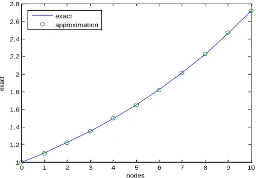
Numerical results are given in Table 1. In this table, the exact and the computed solutions together with the related absolute errors at points have been given. As seen the the computed solution is in good agreement with the exact solution.

The behavior of the approximate solution using Chebyshev polynomials and exact solution are presented in Fig. 2. It is clear that the proposed method can be considered as an efficient method to solve the linear integral equations.

Fig. 2 Approximate and exact solution for Example 1.

0 1 2 3 4 5 6 7 8 9 10

1 1.2 1.4 1.6 1.8 2 2.2 2.4 2.6 2.8

nodes

e

x

a

c

t

International Journal of Basic & Applied Sciences IJBAS-IJENS Vol:16 No:06 26 Example2. Consider the following Fredholm Urysohn

integral equation [1]

( ) ( ) ∫ ( ) _{( ) ( )}

where ( ) ( ) ( ( )) ( ) _{( ), such that the exact solution of the equation is} ( ) . We apply the suggested method with , and approximate the solution x(t) as follows

( ) ∑ ( ) ( ) ( )

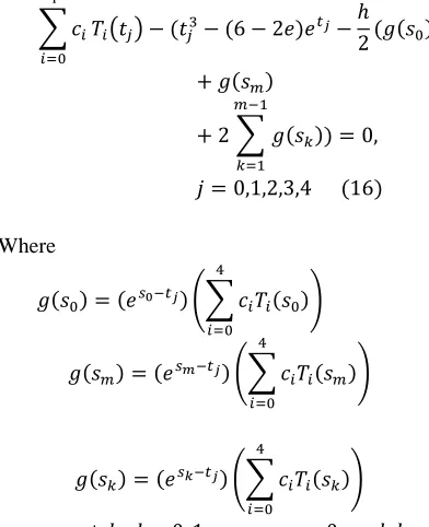
By the same procedure in the previous section and using Eq. (9) we have

∑

( ) ( ( ) ( ( )

( )

∑ ( ))

( )

Where

( ) ( _{) (∑ ( )}

)

( ) ( _{) (∑ ( )}

)

( ) ( _{) (∑ ( )}

)

in which Eq. (16) represents a system of ( ) nonlinear algebraic equations with unknowns . By using the Newton iterative method and initial guess , we obtain:

Therefore, the approximation solution of this example by using

( ) ∑ ( )

is given by

( ) ( ) ( ) ( ) ( ) ( )

TABLE II

EXACT AND APPROXIMATE SOLUTION AND ERROR FOR EXAMPLE 2.

Nodes Exact

solution

Approximate

solution Error

0 0 -5.5511e-17 5.55E-17

1 0.001 -0.0020914 3.09E-03

2 0.008 0.0068374 1.16E-03

3 0.027 0.027832 -8.32E-04

4 0.064 0.06511 -1.11E-03

5 0.125 0.125 0.00E+00

6 0.216 0.21489 1.11E-03

7 0.343 0.34217 8.30E-04

8 0.512 0.51316 -1.16E-03

9 0.729 0.73209 -3.09E-03

10 1 1 0.00E+00

Numerical results are given in Table 2. In this table, the exact and the computed solutions together with the related absolute errors at points have been given. As seen the the computed solution is in good agreement with the exact solution.

The behavior of the approximate solution using Chebyshev polynomials and exact solution are presented in Fig. 3. It is clear that the proposed method can be considered as an efficient method to solve the linear integral equations.

Fig. 3 Approximate and exact solution for Example 2.

0 1 2 3 4 5 6 7 8 9 10

-0.2 0 0.2 0.4 0.6 0.8 1 1.2

nodes

e

x

a

c

t

International Journal of Basic & Applied Sciences IJBAS-IJENS Vol:16 No:06 27

V. CONCLUSION

An approximate method for the solution of linear and nonlinear Fredholm Urysohn integral equations in the most general form has been proposed and investigated. A comparison of the exact and computed solutions reveals that the presented method is effective and convenient. The numerical results show that the accuracy can be improved by increasing N. As observed the method provides a suitable solution to the problem. This approach is useful because of Chebyshev polynomials properties. Due to the large number of calculations, the accuracy of the kernel coefficients are very sensitive to the round – off error in the Chebyshev method.

REFERENCES

[1] Ahmad Jafarian, Zahra Esmailzadeh, On the numerical solution of Urysohn integral equations using Legendre approximation, Journal of Mathematical MODELING. Vol. 1 No.1 (2013) 76–84. [2] M.M. Khader, N.H. Sweilam and W.Y. Kota, On the numerical

solution of Hammerstein integral equations using Legendre approximation, Intern. J. Appl. Math. Bioinform. 1 (2012) 65–76. [3] M.M. Khader and A.S. Hendy, The approximate and exact

solutions of the fractional order delay differential equations using Legendre pseudospectral method, Intern. J. Pure Appl. Math. 74 (2012) 287–297.

[4] M.M. Khader, N.H. Sweilam and A.M.S. Mahdy, An Efficient numerical method for solving the Fractional discussion equation, J. Appl. Math. Bioinform. 1 (2011) 1–12.

[5] M.M. Khader, Introducing an ecient modification of the homotopy perturbation method by using Chebyshev polynomials, Arab J. Math. Sci. 18 (2012) 61–71.

[6] Saran, N., Sharma, S. D. and Trivedi, T. N. 2000. Special Functions, Seventh edition, Pragati Prakashan

[7] Z. Mahmmodi, J. Rashidian and E. Babolian, Spline Collocation for nonlinear Fredholm integral equations, Intern. J. Math. Model. Comput. 1 (2011) 69-75.

[8] A. Jerri, Introduction to integral equations with applications. John Wiley & Sons, 1999.

[9] A. Jafrian, S. A, Measoomy, Alreza K. Golmank Haneh, D. Baleanu. A numerical Solution of the Urysohn-Type Fredholm integral equations. Rom. Journ. Phys., Vol. 59, Nos. 7-8, P.625-635, Bucharest, 2014.