Inference for the shape parameter of lognormal distribution in presence of fuzzy data

Inference for the Shape Parameter of

Lognormal Distribution in Presence of Fuzzy Data

Abbas Pak

Department of Computer Sciences, Faculty of Mathematical Sciences Shahrekord University, P. O. Box 115, Shahrekord, Iran

[email protected], [email protected]

Abstract

Traditional Statistical analysis of lognormal distribution have been proposed for precisely defined crisp data. But there are many other situations in which measurement results from continuous quantities are not precise numbers but more or less fuzzy. This article presents the statistical inference on the shape parameter of lognormal distribution involving experiment whose observations are described in terms of fuzzy data. The maximum likelihood procedure are developed for estimating the unknown parameter. Asymptotic distribution of maximum likelihood estimator is used to construct approximate confidence interval. Also, Bayes estimate and the corresponding highest posterior density credible interval of the unknown parameter are obtained by using Markov Chain Monte Carlo technique. In addition, we describe an estimation method based on moments of lognormal distribution. Extensive simulations are performed to compare the performances of the different proposed methods.

Keywords: Fuzzy data analysis, Lognormal distribution, Maximum likelihood principle, Bayesian estimation, Credible interval.

1. Introduction

Lognormal distribution is one of the distributions commonly used for modeling lifetimes or reaction-times, and is particularly useful for modeling data which are long-tailed and positively skewed. It has been discussed extensively by many authors including Johnson et al. (1994), and Rukhin (1984). Let Y be the original lifetime variable that follows a lognormal distribution with parameters  and  . The density of Y is given by





1 exp ) (2

1 = ) , ;

( _ ₂  2_    

 

 

 y y

y y

f (1)

where  and  are the scale and shape parameters, respectively. In the analysis of lifetime data, it is more convenient to work with the equivalent model for the log-lifetimes. Consider the random variable X =logY . Then, the variable X is normally distributed with density

0. > , ,

2 1 exp ) (2

1 = ) ;

( ₂ 2 

 



   

  



 x x

x

f (2)

presented exact inference procedures (hypotheses tests and confidence intervals) concerning the mean of lognormal distribution by using generalized p-values.

The above inference techniques for estimating the parameters of lognormal distribution are based on precisely defined crisp data. However, in many practical situations we face data which are not only random but vague as well. Randomness involves only uncertainties in the outcomes of an experiment; vagueness, on the other hand, involves uncertainties in the meaning of the data. As an example, consider an opinion poll during which a number of individuals are questioned on their perception of the relative length of different line segments with respect to a fixed longer segment that was used as a standard for comparison. The answers given by the individuals may be vague statements such as “approximately lower than 45 ”, “approximately 50 to 55 ”, “approximately 60 to 65 but near to 65 ”, “approximately higher than 70 ”, and so on. In this situation, randomness occurs when the individuals are selected at random and vagueness is due to meaning of the answer. Classical statistical procedures are not appropriate to deal with such imprecise cases. Fuzzy numbers are well used to model the imprecision of data. A fuzzy number is a subset, denoted by ~ , of the set of real numbers (denoted by x ) and is characterized by the so called membership function ~_x(.). For more details about the fuzzy numbers and probability measures of fuzzy sets, one can refer to Dubois and Prade (1980) and Singpurwalla and Booker (2004).

The rest of this paper is organized as follows. In Section 2, we obtain the maximum likelihood estimate of the parameter  and also construct the approximate confidence interval by using asymptotic normality of the MLE. The Bayesian analyses are presented in Section 3. In Section 4, the estimation via method of moments is provided. Extensive simulations are performed in Section 5 to compare the performances of the MLE, Bayes and moment estimates.

2. ML estimation and confidence interval

Suppose that n identical units are placed on a life test with the corresponding lifetimes n

X

X₁,..., . It is assumed that these variables are independent and identically distributed with density given in (2). Consider the situation where the available information about the lifetime of these experimental units can not be exactly perceived, but that rather it may be assimilated with fuzzy numbers x~₁,...,~x_n with the corresponding membership functions (.),..., ~ (.)

1 ~

n x

x 

 . Based on the fuzzy numbers x~₁,...,x~_n and by using Zadeh’s definition of the probability of a fuzzy event (Zadeh (1968)), we can obtain the likelihood function of  as

. ) ( 2

1 exp 2

1 =

) ~ ,..., ~ ;

( ₂ 2 ~

1 =

1 x x x dx

x L

i x n

i

n _  

 

  

 





Thus, the corresponding log-likelihood function L*()=logL(;~x₁,...,~x_n) becomes

. ) ( 2

1 exp 2 1 log log

= )

( 2 ~

2 1

= *

dx x x

n L

i x n

i

 

 

 

  

  







The maximum likelihood estimate of the parameter  can be carried out by maximizing the observed-data log-likelihood (4). Equating the derivative of the log-likelihood L*() with respect to  to zero, we have

0. = ) ( 2

1 exp

) ( 2

1 exp =

) (

~ 2 2

~ 2 2 3

2

1 = *

dx x x

dx x x

x n

L

i x

i x n

i 



  

 



   

 

   

  

 









In the Newton-Raphson algorithm, the solution of likelihood equation (5) is obtained through an iterative procedure. In each iterative step, the correction  to the previous estimate ₀ produces new estimate ˆ as ˆ =₀. The iteration method is based on Taylor series expansion of the estimating equation (5) in the neighborhood of the previous estimate. Neglecting power of  above the first order and using Taylor’s theorem, we get the following equation which needs to be solved for :

0 * 0 * 2 2 | ) ( = ) (    

 L L

     (6)

where the notation A|₀, for any partial derivative A, means the partial derivative evaluated at ₀. The second-order derivative of the log-likelihood with respect to the parameter, required for proceeding with the Newton-Raphson method, is obtained as

. ] ) ( 2 exp ) ( 2 exp [ ) ( 2 exp ) ( 2 exp 3 = ) ( 2 ~ 2 2 ~ 2 2 3 2 ~ 2 2 ~ 2 2 4 2 6 4 1 = 2 * 2 2                                                     











The maximum likelihood estimate of  via Newton-Raphson algorithm is thereafter refereed as “ˆ ” in this paper. Once the maximum likelihood estimate of NR  is obtained, we can use the asymptotic normality of the MLEs to construct the approximate confidence interval. It is known that the asymptotic distribution of the MLE of  is given by, see Miller (1981),

)). ( (0, )

ˆ

(_NR N Var 

Here, the asymptotic variance Var() can be approximated as

, ) ˆ ( 1 ) ˆ ( NR NR I Var   

where I(ˆNR) denotes the observed Fisher information given by . | ) ( = ) ˆ

( ₂ * _=ˆ

2

NR

NR L

I  _{ }

 

  

Thus, the approximate 100(1)% confidence interval for the parameter  can be computed as:





L   z Var 

  _

where

2 

z is an upper percentile of the standard normal variate.

3. Bayesian estimation

as follows: ₂

2 1 =



 . Based on the new parametrization, we consider the Bayesian estimation of . In this case, the likelihood function (3) can be reexpressed as





1 = )

( 2 ~

1 = 2

dx x x

L

i x n

i n

  



  

    





In many practical situations, it is observed that the behavior of the parameters representing the various model characteristics cannot be treated as fixed constant throughout the life testing period. Therefore, it would be reasonable to assume that the parameters involved in the model behave as random variables with distribution commonly known as prior probability distribution. Keeping in mind this fact, we conduct a Bayesian study by assuming the following gamma prior for :

0. > 0, > 0, > ), ( exp )

( a1 b  a b

   

(9)

By combining (8) with (9), the joint density function of the data and  becomes





) ( exp )

, ~ ,..., ~

( 2 ~

1 = 1

2

1 x b x x dx

x

i x n

i a

n

n     

    





Thus, the posterior density function of  given the data can be obtained as

. ) , ~ ,..., ~ (

) , ~ ,..., ~ ( = ) ~ ,..., ~ | (

1 0

1 1

  

 

 

d x x

x x x

x

n n n





(11)

It is well established that the Bayes estimate of any function of , say h()= , under squared error loss function is the posterior mean which is obtained by

. ) ( ) ~ ,..., ~ |

( ₁

0

  

 x x_n h d





(12)

The Eqs. (11) and (12) do not simplified to nice closed forms due to the complex form of the likelihood function. Therefore, we propose a Markov Chain Monte Carlo (MCMC) technique to compute the Bayes estimate of  and also construct its HPD credible interval. Note that the density function (|~x₁,...,~x_n) is not known, but by experimentation, we observed that it is similar to normal distribution. So to generate random samples from posterior density (|~x1,...,~xn), we can use the Metropolis– Hastings algorithm with normal proposal distribution. Thus, the algorithm of MCMC is as follows:

Step 2) Generate _j from (|~x₁,...,x~_n) using Metropolis-Hastings algorithm with the proposal distribution g()I(>0)N(ˆ,1), where I(.) is the indicator function and ˆ is the MLE of , as follows:

(a) Let =j1.

(b) Generate  from the proposal distribution g.

(c) Let

   

 

) ( ) ~ ,..., ~ | (

) ( ) ~ ,..., ~ | ( 1, min = ) , (

1 1

 



 

 



q x x

q x x p

n

n _.

(d) Accept  with probability p(,) or accept  with probability 1p(,). Step 3) Repeat Step 2, M times and obtain _j and _j =h(_j) for j=1,...,M.

Step 4) The Bayes estimate of  , say ˆ , with respect to squared error loss function can _B be obtained as

). ( 1 = ˆ

1 =

j M

t

B h

M 





Step 5) Arrange _j for j=1,...,M , say ₍₁₎ <...<₍M₎ and consider the following

)%

100(1 credible intervals of  :

). , ( ),..., ,

((1) ((1)M) (M) (M)

Then, following Chen and Shao (1999), the HPD credible interval can be obtained by choosing the interval which has the shortest length.

4. Moment estimation

Let ~x₁,...,x~_n denote a fuzzy sample of size n from the population given in (2) with (.)

(.),..., ~ 1

~

n x

x 

 being the corresponding membership functions. Then, by equating the second sample moment to the corresponding population moment, the following equation can be used to find the estimate of  based on moment method:

.

) ( 2

exp

) ( 2

exp 1

=

1/2

~ 2 2

~ 2 2 2

1 =

      

      

   

  

   

  







dx x x

dx x x

x n

i x i x n

i _

  

 (13)

Note that Eq. (13) cannot be computed analytically; therefore, in the following, we describe an iterative numerical process to obtain the parameter estimate:

1. Given initial estimate of  , say (0)

2. Starting from h=0, in the (h1)th iteration, the solution for  , say (h1)

, can be obtained through the following equation

 

 

.

) ( 2

exp

) ( 2

exp 1

=

1/2

~ 2 ) (

2

~ 2 ) (

2 2

1 = 1)

(

      

      

    

   

    

   









dx x x

dx x x

x

n

i x h

i x h n

i h

 

 

 (14)

3 . Checking convergence, if the convergence occurs then the current (h1) is the estimate of  by the method of moments; Otherwise set h=h1 and go to Step 2. The resultant estimate of  is thereafter refereed as “ MME” in this paper.

5. Simulation study and comparisons

In this section we present some simulation results to compare the performances of the different methods proposed in the previous sections. We mainly compare the performances of the MLE, Bayes and moment estimates of the unknown parameter, in terms of their average biases and mean squared errors. We also compare the average lengths of the confidence and credible intervals and their coverage percentages. All the computations are performed on R 2.11.0.

For simulation purposes, we have considered different choices of sample sizes n and fixed value of the parameter, namely  =1. In each case, we have generated fuzzy random sample from the distribution given in (2) by using the algorithm given in Pak et al. (2014) which involves the following steps:

1) Generate n independent and identically distributed (iid) random numbers

1

( ,...,u u_n)from uniform distribution U(0,1).

2) Set x_i  1( )u_i , i 1,...,n, where  is the cumulative distribution function of normal distribution. Now, (x₁,...,x_n) is a sample of size n from standard normal distribution.

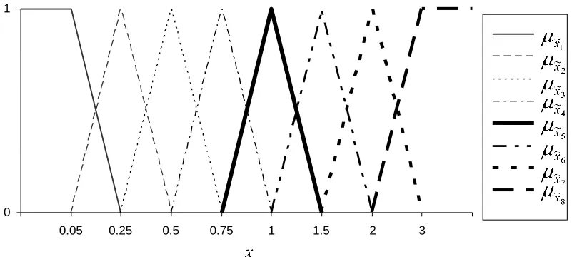
3) Consider the fuzzy information system shown in Fig.1, corresponding to the membership functions

  

  

 

  

  

    

 

 

, 0

0.5, 0.25

0.25 0.5

0.25, 0.05

0.2 0.05 =

) ( ,

0

0.25, 0.05

0.2 0.25

0.05, 1

= ) (

2 ~ 1

~

otherwise x x

x x

x otherwise

x x

x

x _x

x



                            , 0 1, 75 . 0 0.25 1 75, . 0 0.5 0.25 0.5 = ) ( , 0 75, . 0 0.5 0.25 75 . 0 0.5, 0.25 0.25 0.25 = ) ( 4 ~ 3 ~ otherwise x x x x x otherwise x x x x x _x x                               , 0 2, 1.5 0.5 2 1.5, 1 0.5 1 = ) ( , 0 1.5, 1 0.5 1.5 1, 75 . 0 0.25 75 . 0 = ) ( 6 ~ 5 ~ otherwise x x x x x otherwise x x x x x _x x                         . 0 3, 1 3, 2 2 = ) ( , 0 3, 2 3 2, 1.5 0.5 1.5 = ) ( 8 ~ 7 ~ otherwise x x x x otherwise x x x x x _x x  

4) For each generated sample in step 2, select the membership function that best describes the realization x_i .

Then, the estimate of the parameter  for the fuzzy sample were computed using the maximum likelihood method, Bayesian procedure and moment method. In computing the MLE, we have used the true value of  as the initial guess value of  in the Newton-Raphson algorithm. For computing the Bayes estimate, we have assumed non-informative gamma prior, i.e. a=b=0, and also informative gamma prior, i.e.

2 = =b

a . We replicate the process 10000 times and report the average biases (AB) and mean squared errors (MSE) of the estimates in Tables 1 and 2.

Figure 1: Fuzzy information system used to encode the simulated data

0 1

We have also computed approximate 95% confidence interval and the HPD credible interval of the unknown parameter. Criteria appropriate to the evaluation of the two methods under scrutiny include: closeness of the coverage probability to its nominal value and expected interval width. For each simulated sample, we have computed confidence/credible intervals and checked whether the true value of the parameter lay within the intervals and recorded the length of the intervals. The estimated coverage probability was computed as the number of intervals that covered the true value divided by 10000 while the estimated expected width of the intervals was computed as the sum of the lengths for all intervals divided by 10000. The coverage probabilities and the expected widths for different sample sizes are presented in Tables 1 and 2.

Table 1: Averages biases and mean squared errors of the ML and moment estimates of , coverage probabilities and expected width of the confidence interval

n

MLE MME Confidence interval

AB MSE AB MSE Coverage Length

15 0.0619 0.0385 0.0620 0.0386 0.9345 0.7640

20 0.0537 0.0329 0.0539 0.0330 0.9437 0.6783

30 0.0488 0.0273 0.0488 0.0273 0.9482 0.5545

50 0.0353 0.0214 0.0355 0.0215 0.9504 0.4266

70 0.0281 0.0158 0.0282 0.0159 0.9516 0.3617

100 0.0244 0.0136 0.0244 0.0136 0.9534 0.2978

Table 2: Averages biases and mean squared errors of the Bayes estimates of  , coverage probabilities and expected width of the credible interval for different priors

n

Non-informative prior (a=b=0) Informative prior (a=b=2)

Bayes estimate Credible interval Bayes estimate Credible interval

AB MSE Coverage Length AB MSE Coverage Length

15 0.0612 0.0379 0.9374 0.7491 0.0544 0.0331 0.9431 0.7265 20 0.0528 0.0327 0.9450 0.6637 0.0485 0.0308 0.9472 0.6513 30 0.0473 0.0272 0.9493 0.5405 0.0356 0.0229 0.9503 0.5284 50 0.0346 0.0210 0.9508 0.4118 0.0298 0.0174 0.9518 0.3825 70 0.0279 0.0158 0.9523 0.3459 0.0243 0.0125 0.9537 0.2991

100 0.0242 0.0131 0.9539 0.2813 0.0218 0.0106 0.9556 0.2676

Now considering the confidence and credible intervals, it is observed that the asymptotic results of the MLE work quite well, even when the sample size is small. It can maintain the coverage percentages in most of the cases. The widths of the confidence/credible intervals narrow down with an increase in the sample size n. The performance of the credible intervals are satisfactory and their coverage percentages are close to the corresponding nominal level. Moreover, it is seen that an informative prior distribution improves the performance of the Bayesian credible interval compared to the one using non-informative prior.

6. Conclusion

In this paper, we have developed inferential procedures for the shape parameter of lognormal distribution when the available observations are fuzzy and are assumed to be related to underlying crisp realization of a random sample. In particular, we have used the Newton-Raphson algorithm to determine the maximum likelihood estimate of the parameter. For computing the Bayes estimate, we have used Markov Chain Monte Carlo method with different types of prior information. Also, the estimation via moments method has been presented by an iterative process. We have further constructed approximate confidence interval and HPD credible interval of the unknown parameter. The performances of the different methods have been compared by Monte Carlo simulations. Based on the results of the simulation study, we see clearly that, the performances of the ML and moment estimates are very similar in all aspects. Also, the Bayes estimates based on non-informative prior and maximum likelihood estimates give similar estimation results; however, the Bayes estimates with informative prior have smaller MSE, showing that additional prior information about the parameter  provides an improvement in the estimates. The AB and MSE of all the estimators decrease significantly as the sample size n increases, as one would expected. It can be further observed that, in most of the cases, the coverage probabilities of confidence/credible are close to the nominal level and theier average lengths also decrease as n increases. Finally, it should be mentioned that Bayes estimates are more computationally expensive than the MLEs and MMEs.

References

1. Balakrishnan, N., and Mitra, D. (2011). Likelihood inference for lognormal data with left truncation and right censoring with an illustration. Journal of Statistical Planning and Inference, 141, 3536-3553.

2. Basak, P., Basak, I. and Balakrishnan, N. (2009). Estimation for the three-parameter lognormal distribution based on progressively censored data. Computational Statistics & Data Analysis, 53(10), 3580-3592.

3. Chen, M.H. and Shao, Q.M. (1999). Monte Carlo estimation of Bayesian credible and HPD intervals. Journal of Computational and Graphical Statistics, 8(1), 69-92.

5. Dubois, D. and Prade, H. (1980). Fuzzy Sets and Systems: Theory and Applications. Academic Press, New York.

6. Gil M.A., López-Diaz M., Ralescu D.A. (2006), Overview on the development of fuzzy random variables, Fuzzy Sets and Systems, 157(19), 2546-2557.

7. Johnson, N.L., Kotz, S. and Balakrishnan, N. (1994). Continuous Univariate Distributions-vol. 1, second ed. John Wiley & Sons, New York.

8. Krishnamoorthy, K., and Mathew, T., (2003). Inferences on the means of lognormal distributions using generalized p-values and generalized confidence intervals. Journal of Statistical Planning and Inference, 115, 103-121.

9. Longford, N.T., (2009). Inference with the lognormal distribution. Journal of Statistical Planning and Inference, 139(7), 2329-2340.

10. Miller, R.C., (1981). Survival analysis, John Wiley& Sons.

11. Pak, A., Parham, G.H. and Saraj, M., (2013). Inference for the Weibull Distribution Based on Fuzzy Data. Revista Colombiana de Estadistica, 36(2), 339-358.

12. Pak A, Parham GA and Saraj M. (2014). Inferences on the Competing Risk Reliability Problem for Exponential Distribution Based on Fuzzy Data. IEEE Transactions on reliability, 63(1), 2-13.

13. Rukhin, A.L. (1984). Improved estimation in lognormal models. Technical Report No. 84-38, Department of Statistics, Purdue University, West Lafayette, Indiana.

14. Singpurwalla, N.D., and Booker, J.M., (2004). Membership functions and probability measures of fuzzy sets, Journal of the American Statistical Association, 99(467), 867–877.

15. Viertl R. (2006). Univariate statistical analysis with fuzzy data. Computational Statistics & Data Analysis, 51(1), 133-147.

16. Wu, H.C. (2004). Fuzzy Bayesian estimation on lifetime data. Computational Statistics, 19, 613-633.

17. Zadeh, L. A. (1968). Probability measures of fuzzy events, Journal of Mathematical Analysis and Applications. 10, 421-427.