Stability and Hopf Bifurcation Analysis of Delayed Rosenzweig-MacArthur Model with Prey Immigration

http://www.sciencepublishinggroup.com/j/cssp doi: 10.11648/j.ajam.20190706.14

ISSN: 2330-0043 (Print); ISSN: 2330-006X (Online)

Stability and Hopf Bifurcation Analysis of Delayed

Rosenzweig-MacArthur Model with Prey Immigration

Gang Zhu

∗

_{, Chunyan He}

School of Education Science, Harbin University, Harbin, P. R. China

Email address:

[email protected] (Gang Zhu)

To cite this article:

Gang Zhu, Chunyan He. Stability and Hopf Bifurcation Analysis of Delayed Rosenzweig-MacArthur Model with Prey ImmigrationAmerican Journal of Applied Mathematics. Vol. 7, No. 6, 2019, pp. 164-176. doi: 10.11648/j.ajam.20190706.14

Received:October 25, 2019;Accepted:November 18, 2019;Published:December 30, 2019

Abstract:

A delayed reaction Cdiffusion Rosenzweig-MacArthur model with a constant rate of prey immigration is considered. We derive the characteristic equation through partial differential equation theory, and by analyzing the distribution of the roots of the characteristic equation, the local stability of the positive equilibria is studied, and we get the conditions to determine the stability of the positive equilibria. Furthermore we find that Hopf bifurcation occurs near the positive equilibrium when the time delay passes some critical values, and we get the conditions under which the Hopf bifurcation occurs and so periodic solutions appear near the positive equilibria. By using the center manifold theory and normal form method, we derive an explicit algorithm for determining the direction of the Hopf bifurcation and the stability of the bifurcating periodic solutions. Furthermore, some numerical simulations are carried out to illustrate the analytic results of our study.

Keywords:

Delay, Stability, Bifurcation, Center Manifold, Normal Form

1. Introduction

Predator-prey systems (or consumer-resource systems) are basic differential equation models for describing the interactions between two species with a pair of positive-negative feedbacks. Furthermore, many ecological concepts such as diffusion, functional responses and time delays have been taken into consideration to gain more accurate description and better understanding [1-6]. A typical Rosenzweig-MacArthur model was put forward first in [7]. In this model the prey has a logistic growth and the predator has a Holling

II functional response. In [8-12] the global stability are discussed. There are also many researches on the limit cycle of R-M model [13-16]. In [17], Malay Banerjeethe studied the existence of Turing patterns in this model and in the effect of the non-local interaction on the periodic travelling wave and spatio-temporal chaotic patterns. In [18], a fractional order Rosenzweig-MacArthur (R-M) model incorporating a prey refuge is constructed and analyzed in detail. Sugie et al discussed the existence and uniqueness of limit cycles in predator-prey systems with a constant immigration in [19].

In this paper, we study the reaction-diffusion system, Rosenzweig-MacArthur model with a constant immigration.

∂u(t, x)

∂t =D14u(t, x) +ru(t, x)

1−u(t, x)

k

−u(t, x)v(t, x)

a+u(t, x) +b

∂v(t, x)

∂t =D24v(t, x)−dv(t, x)+

µu(t−τ, x)v(t−τ, x)

a+u(t−τ, x) , x∈Ω, t >0

∂u(t, x)

∂ν =

∂u(t, x)

∂ν = 0, (1)

WhereΩ = (0, π), the homogeneous Neumann boundary condition means the system is a closed one. u(t, x), v(t, x)

stand for the densities of the prey and predator at timet > 0

and a spatial positionx ∈ Ω,D1, D2 > 0 are the diffusion

coefficients of the species. a, b, d, k, r, µ are all positive constants, and the meaning of them are the same as those in [19], andτ ≥ 0is the constant delay due to the gestation of the predator.

It is easy to see that system (1) always has a boundary equilibrium

E0(u0,0) =

k

2 +

√

k2_r2_{+ 4bkr}

2r ,0

!

Whenµ > d, we let

R0=

bk(µ−d)2+adkr(µ−d)

a2_d2_r

then we can get that when R0 ≤ 1 system (1) has no

positive equilibrium andE0(x0,0)is the unique equilibrium

of (1) ; and when R0 > 1 system (1.1) has a positive

equilibriumE∗(u∗, v∗)besidesE0(u0,0),

E∗(u∗, v∗) =

_ad

µ−d, µ d

h

ru∗

1−u∗

k

+bi

By straightforward calculation, we get the characteristic equation of the linearizing system of (1) about E0

λ+D1n2−r

1−2u0

k

λ+D2n2+d−

µu0

a+u0

e−λτ

= 0

Similar to the discussion in [20], we know thatE0is locally

asymptotically stable whenR0 <1, and unstable whenR0 >

1.

The rest of the present paper is organized as follows: In Section 2, we analyze the local stability of the positive equilibriumE∗, and the existence of Hopf bifurcation atE∗.

In section 3, we determine the properties of the bifurcating periodic solution. In Section 4, some numerical simulations are carried out to illustrate the analytic results.

2. Local Stability of

E

∗

and the Existence

of Hopf Bi-furcation

As shown in section 1, we know that system (1) has a positive equilibrium E∗(u∗, v∗) when R0 > 1.

MoveE∗(u∗, v∗)to the originO(0,0), we can rewrite (1) as

follow:

∂u(t, x)

∂t =D14u(t, x) +α1u(t, x)−α2v(t, x) +f1(u, v)

∂v(t, x)

∂t =D24v(t, x)− dv(t, x) +β1u(t−τ, x) +dv(t−τ, x) +f2(u, v)

∂u(t, x)

∂ν =

∂u(t, x)

∂ν = 0, x∈∂Ω, t≥0u(t, x) =φ(t, x)−u∗, v(t, x) =ψ(t, x)−v∗, x∈Ω¯, θ∈[−τ,0]

(2)

where

α1=r−

2ru∗

k − av∗

(a+u∗)2

, α2=

u∗

a+u∗

, β1=

aµv∗

(a+u∗)2

f1(u, v) =−

ru(t, x)2

k +

av∗u2(t, x)−a(a+u∗)u(t, x)v(t, x)

(a+u∗)2(a+u∗+u(t, x))

f2(u, v) =aµ

(a+u∗)u(t−τ, x)v(t−τ, x)−v∗u2(t−τ, x)

(a+u∗)2(a+u∗+u(t−τ, x))

(3)

DenotinigX =C([0, π],_R2_{), C}

τ=C([−τ,0], X)

u1=u(t,·), u2=v(t,·), U = (u1, u2)T

then we can write (2) as an abstract ordinary differential equation in the phase spaceCτ

˙

U(t) =D4U(t) +L(Ut) +F(Ut) (4) where

dom(D4) ={(u, v)T|u, V ∈C2([0, π],_R), ∂νu=∂νv= 0, π}

L(φ) =

α1 −α2

0 0

φ1(0)

φ2(0)

+

0 0

β1 d

φ1(−τ)

φ2(−τ)

, D=

D1 0

0 D2

F(φ) =



  

−rφ

2 1(0)

k +

av∗φ21(0)−a(a+u∗)φ1(0)φ2(0)

(a+u∗)2(a+u∗+φ1(0))

aµ(a+u∗)φ1(−τ)φ2(−τ)−v∗φ

2 1(−τ)

(a+u∗)2(a+u∗+φ1(−τ))



  

Equation (4) has the linear part

˙

U(t) =D4U(t) +L(Ut)

and the characteristic equation

λy−D4y−L(eλ·y) = 0, y∈dom(D4)\{0}

Letting

φ=

∞

X

n=0

an bn

!

cos(nπx)

be the characteristic function corresponding to the eigenvaluesλ, then the characteristic equation has the following form

4n(λ, τ) =λ2+Anλ+Bn+ (Cn−dλ)eλτ = 0, (5)

where

An = (D1+D2)n2+d−α1,

Bn =D1D2n4+ (D1d−D2α1)n2−dα1,

Cn =−D1dn2+dα1+α2β1.

Assuming condition(A)as follow:

(A) α1<0⇔r+

adr kµ <

2adr k(µ−d)+

r(µ−d)

µ +

b(µ−d)2

adµ ,

then we haveLemma 2.1.If(A)holds, thenλ= 0is not the root of Eq. (5) for anyn∈N0.

Proof.According to (5) we know that

4n(0, τ) =Bn+Cn=D2n2(D1n2−α1) +α2β1

Condition(A)holds means thatα1<0, and from (3) we can getα2>0, β1>0, then

4n(0, τ)>0,∀n∈N0.

Lemma 2.2. If(A)holds, whenτ= 0, all roots of Eq. (5) have negative real parts,for anyn∈N0, furthermore,E∗is locally

asymptotically stable.

Proof.Whenτ= 0, Eq. (5) becomes

4n(λ,0) =λ2+ (An−d)λ+Bn+Cn= 0.

Suppose thatλ1n, λ2nbe roots of the above equation, then we have

λ1n+λ2n=d−An=α1−(D1+D2)<0

λ1nλ2n=Bn+Cn=D1D2n4−D2α1n2+α2β1>0,

which completes the proof.

Whenτ 6= 0, lettingıω(ω >0)be the root of Eq.(5), then

Cnsinωτ +dωcosωτ =Anω Cncosωτ−dωsinωτ =ω2−Bn

which leads to

Letz=ω2, Eq. (6) becomes

z2+ (A2n−2Bn−d

2

)z+Bn2−C

2

n= 0. (7)

Through calculation we know that

A2_n−2Bn−d2= [(D1+D2)n2+d−α1]2−2[D1D2n4+ (D1d−D2α1)n2−dα1]−d2,

=D2n4+ 2D2dn2+ (D1n2−α1)2>0,

Bn2−Cn2= (Bn+Cn)(Bn−Cn), Bn+Cn=D1D2n4−D2α1n2+α2β1,

Bn−Cn=D1D2n4+ (2D1d−D2α1)n2−2α1d−α2β1.

Suppose condition(A)holds. It is obvious thatBn+Cn>0. Furthermore, if−2α1d−α2β1>0, thenBn−Cn>0, ∀ n∈ N0; if−2α1d−α2β1 < 0, sinceB0−C0 = −2α1d−α2β1 < 0, then there existsN ∈ N, such thatBn−Cn <0 when n < Nand Bn−Cn >0when n > N. So we get that if(A)and−2α1d−α2β1>0hold, then Eq. (7) has no positive root

for∀n∈_N0; and if(A)and−2α1d−α2β1<0hold, Eq. (7) has a positive root

zn =1

2[2Bn+d

2_−A2

n+

p

(A2

n−2Bn−d2)2−4(B2n−Cn2)] whenn < N, which means that Eq. (6) also has a positive root

ωn= √1

2

q

2Bn+d2_−A2

n+

p

(A2

n−2Bn−d2)2−4(Bn2−Cn2)

Lemma 2.3. If(A)and−2α1d−α2β1 < 0hold, then there existN ∈ N, such that Eq. (5) has a pair of conjugate pure imaginary roots ±ıωnwhenτ =τnj(n < N, j= 0,1,2,· · ·), where

τ_nj =

   

  

1

ωn

arccosa

∗

c∗ + 2jπ

, b∗>0 1

ωn

2π−arccosa

∗

c∗ + 2jπ

, b∗<0

(8)

herea∗= (dAn+Cn)ω2_{−BnCn, b}∗_{=ω(AnCn−dBn)−dω}3_{, c}∗_=C2

n+d2ω2. Furthermore, we haveLemma 2.4.Re(dλ/dτ)|_τ=τj

n>0 Proof.Since (5), we know that

[2λ+An−de−λτ−τ(Cn−dλ)λe−λτ]dλ

dτ = (Cn−dλ)λe

−λτ_,

which leads to

_dλ

dτ

−1

=2λ+An−de

−λτ

λ(Cn−dλ)e−λτ

−τ

λ

= 2λ+An

−λ(λ2_+Anλ+Bn)−

d λ(Cn−dλ)−

τ λ,

substitutingτ =τ_njinto the above formula, we have

Re

dλ

dτ

−1

τ=τnj

= Re

2ıωn+An

−ıωn(−ω2

n+ ıωnAn+Bn)

− d

ıωn(Cn−ıdωn)−

τnj

ıωn

= A

2

n+ 2(ω2n−Bn) A2

nω2n+ (ωn2−Bn2)2

− d

2

d2_ω2

n+Cn2

= A

2

n−2Bn−d2+ 2ωn2 d2_ω2

n+Cn2

>0.

(i)If−2α1d−α2β1>0, thenE∗(u∗, v∗)is locally asymptotically stable for∀τ∈[0,+∞);

(ii)If−2α1d−α2β1<0, thenE∗(u∗, v∗)is locally asymptotically stable whenτ ∈[0, τ∗)and unstable whenτ > τ∗; and

system undergoes Hopf bifurcation atE∗(u∗, v∗)whenτ =τnj(0≤n < N, j= 0,1,2,· · ·). The bifurcating period solutions are spatially homogenous whenτ=τ₀j(j= 0,1,2,· · ·); The bifurcating period solutions are spatially non-homogenous whenτ=τj

n(0< n < N, j= 0,1,2,· · ·).

3. Properties of Hopf Bifurcation

Basing on the discussion in the previous section, we find that under some condition system (1) undergoes Hopf bifurcation, which means that system (1) has bifurcating period solutions. This section, using theory of partial differential equation from Wu [26] and Hassard [27], we study the properties of bifurcating period solutions.

Lettingu¯(t, x) =u(τ t, x), v¯(t, x) = v(τ t, x), and removing the”−”for convenience, expanding system (2) around the origin, we get the following equation:

∂u(t, x)

∂t =τ D14u(t, x) +τ[α1u(t, x)−α2v(t, x) +α3u

2_{(t, x) +α}

4u(t, x)v(t, x)

+α5u3(t, x) +α6u2(t, x)v(t, x) +O(4)]

∂v(t, x)

∂t =τ D24v(t, x) +τ[−dv(t, x) +β1u(t−τ, x) +dv(t−τ, x) +β2u

2_{(t−1, x)}

+β3u(t−1, x)v(t−1, x) +β4u3(t−1, x) +β5u2(t−1, x)v(t−1, x) +O(4)]

(9)

where

α3=−

r k+

av∗

(a+u∗)3

, α4=

−a

(a+u∗)2

, α5=

av∗

(a+u∗)4

, α6=

−a

(a+u∗)3

β2=−

aµv∗

(a+u∗)3

, β3=

aµ

(a+u∗)2

, β4=

aµv∗

(a+u∗)4

, β5=

−aµ

(a+u∗)3

Let

u1(t) =u(t,·), v1(t) =v(t,·), U= (u1, u2)T

then system (9) can be written as the following abstract ordinary differential equation in the phase spaceC=C([−1,0], X) dU(t)

dt = ¯τ D4U(t) +Lτ¯(Ut) +F(Ut, ε) (10) HereL:C7→X, F :C7→Xare defined as

Lε(φ) =ε

α1φ1(0)−α2φ2(0)

−dφ1(0) +β1φ1(−1) +dφ2(−1)

and

F(φ, ε) =εD4φ+Lε(φ) +f(φ, ε)f(φ, ε) = (¯τ+ε)

α3φ21(0) +α4φ1(0)φ2(0) +α5φ31(0) +α6φ21(0)φ2(0) +O(4)

β2φ21(−1) +β3φ1(−1)φ2(−1) +β4φ31(−1) +β5φ12(−1)φ2(−1) +O(4)

₍₁₁₎

whereφ= (φ1, φ2)T ∈C.

Consider the following linear equation

dU(t)

dt = ¯τ D4U(t) +Lτ¯(Ut) (12) Whenτ = ¯τ, system (9) has pure imaginary roots, denoted asΛ ={i¯ωτ ,¯ −i¯ω¯τ}, what’s more,Λare also eigenvalues of the following functional differential equation.

dz(t)

dt =−τ Dn¯

2_{z(t) +L} ¯

By Riesz representation theorem, there exists a 2×2matrix ηn(θ,τ¯) (−1≤θ≤0), whose elements are of bounded variation functions, such that

−τ Dn¯ 2φ(0) +Lτ¯(φ) =

Z 0

−1

dηn(θ,τ¯)φ(θ).

ηn(θ,τ¯) =

     

    

¯

τ

α1 −α2

0 0

, θ= 0 0, θ∈(−1,0) ¯

τ

0 0

β1 d

, θ=−1

For∀φ∈ C ∩C1_{andψ∈ C ∩C}1_{, define the operatorA(ε)andA}∗_{respectively as follow}

A(ε)φ(θ) =

 



dφ(θ)

dθ , θ∈[−1,0),

R0

−1dη(θ, ε)φ(θ), θ= 0,

A∗ψ(s) =

 



−dψ(s)

ds , s∈(0,1],

R0

−1ψ(−ξ)dη(ξ,0), s= 0.

Define the bilinear form

(φ, ψ) =ψ(0)φ(0)−

Z 0

−1

Z θ

ξ=0

ψ(ξ−θ)dηn(θ,τ¯)φ(ξ)dξ

=ψ(0)φ(0) + ¯τ

Z 0

−1

ψ(ξ+ 1)

0 0

β1 d

φ(ξ)dξ

(14)

where φ ∈ C([−1,0],_R2_{), ψ ∈ C([0,1],}

R∗). Then A(0) and A∗ are adjoint operators, and ±i¯ωτ¯ are eigenvalues of A(¯τ)andA∗. LetP andP∗ are center subspaces ofA(¯τ)andA∗ associated withΛ ={±i¯ωτ¯}respectively, thenP∗is the adjoint space ofP, anddimP= dimP∗= 2.

By a straightforward computation, we can get that

p1(θ) = (1, ξ)Tei ¯ω¯τ(θ∈[−1,0]), p2(θ) =p1(θ)

and

q1(s) = (η,1)e−i ¯ωτ¯(s∈[0,1]), q2(s) =p1(s)

are bases ofA(¯τ)andA∗associated withΛ ={±i¯ωτ¯}, where

ξ= 1

α2

(α1−D1n2−i¯ω),

η= 1

α2

[−d−D2n2+dcos ¯ωτ¯+ i(¯ω+dsin ¯ωτ¯)].

Taking

Φ1(θ) =

1

2[p1(θ) +p2(θ)] =

Re(ei ¯ω¯τ θ)

Re(ξei ¯ωτ θ¯ ₎

=





cos(¯ωτ θ¯ ) 1

α2

[(α1−D1n2) cos(¯ω¯τ θ) + ¯ωsin(¯ω¯τ θ)]





Φ2(θ) =

1

2[p1(θ)−p2(θ)] =

Im(ei ¯ω¯τ θ)

Im(ξei ¯ωτ θ¯ )

=





sin(¯ωτ θ¯ ) 1

α2

[(α1−D1n2) sin(¯ωτ θ¯ )−ω¯cos(¯ω¯τ θ)]



and

Ψ∗₁(s) =1

2[q1(s) +q2(s)] = Re(ηe

−i ¯ωτ θ¯ _),

Re(e−i ¯ωτ θ¯ )

=

₁

α2

[(−d−D2n2+dcos(¯ωτ s¯ )) cos(¯ωτ s¯ ) + (¯ω+dsin(¯ωτ s¯ )) sin(¯ω¯τ s)],cos(¯ωτ s¯ )

Ψ∗₂(s) =1

2[q1(s)−q2(s)] = Im(ηe

−i ¯ωτ s¯ _),Im(e−i ¯ω¯τ s₎

=

₁

α2

[(d+D2n2−dcos(¯ωτ s¯ )) sin(¯ω¯τ s) + (¯ω+dsin(¯ωτ s¯ )) cos(¯ωτ s¯ )],−sin(¯ωτ s¯ )

then(Φ1,Φ2)and(Ψ∗1,Ψ∗2)are bases forPandP∗respectively.

By (14), we have

M1:= (Ψ∗1,Φ1) =

1 2α2

[2γ+ ¯τ γρ−dω¯τ¯sin(¯ωτ¯)]

M2:= (Ψ∗1,Φ2) =

−1 2α2

[2¯ω+dω¯τ ρ¯ + ¯τ γsin(¯ωτ¯)]

M3:= (Ψ∗2,Φ1) =

1 2α2

[2¯ω−dω¯τ δ¯ −¯τ γsin(¯ωτ¯)]

M4:= (Ψ∗2,Φ2) =

1 2α2

[¯τ γδ−dω¯¯τsin(¯ωτ¯)]

where

γ=α1−D1n2−D2n2, ρ= cos(¯ωτ¯) +

sin(¯ωτ¯) ¯

ωτ¯ , δ= cos(¯ωτ¯)−

sin(¯ω¯τ) ¯

ωτ¯ .

Define

(Ψ,Φ) = (Ψ∗_j,Φk) =

(Ψ∗₁,Φ1) (Ψ∗1,Φ2)

(Ψ∗2,Φ1) (Ψ∗2,Φ2)

and chooseΨ = (Ψ1,Ψ2)T = (Ψ∗,Φ)−1Ψ∗, then we have(Ψ,Φ) =I2, and

Ψ1(0)−iΨ2(0) =

1

M1M4−M2M3

_−D

2n2

α2

(M3+M4i)−ω¯(M2+M1i), M4+M3i

:= (Υ1,Υ2)

(15)

Takefn = (β1n, βn2), here

β_n1 =

cos(nx) 0

, β_n2=

0 cos(nx)

and denote

c·fn:=c1β1n+c2β2n, c= (c1, c2)T ∈C([−1,0], X)

Foru= (u1, u2), v= (v1, v2), u, v∈X, define inner product as

hu, vi= 1

π

Z π

0

u1¯v1dx+

1

π

Z π

0

u2¯v2dx.

Forφ∈C=C([−1,0], X), definehφ, fni= (hφ, fn1i,hφ, fn2i)T, then we get the center subspace of Eq. (12)

PCNC(φ) = Φ(Ψ,hφ, fki)·fk, φ∈C,

and we can decompose space intoC=PCNC⊕PSC, wherePSCis the complementary space ofPCNCinC.

LetAτ¯be the infinitesimal generator of the semigroup induced by solutions of Eq. (13), then (2) can be written as the abstract

ODE

dU(t)

dt =A¯τUt+R(Ut, ε) (16)

where

R(Ut, ε) =

0, θ∈[−1,0)

We can decompose the abstract equation into

Ut= Φ x1

x2

!

·fn+h(x1, x2, ε),

where

x1

x2

!

= (Ψ,hUt, fni), h(x1, x2, ε)∈PSC, h(0,0,0) = 0, Dh(0,0,0) = 0.

Solutions of (10) on the center manifold are

Ut= Φ x1(t)

x2(t)

!

·fn+h(x1, x2,0) (17)

Letz(t) =x1(t)−ix2(t), then we have

˙

z(t) = i¯ω¯τ z(t) +g(z,z¯)

where

g(z,z¯) = (Ψ1(0)−iΨ2(0))hF(Ut,0), fni

Substitutez(t)into (17), we get

Φ x1(t)

x2(t)

!

·fn= (Φ1,Φ2)



 

z+ ¯z

2 i(z−z¯)

2



 ·fn=

1

2(p1z+ ¯p1z¯)·fn

and

h(x1, x2,0) =h

_{z+ ¯z}

2 ,

i(z−z¯) 2 ,0

thenUtcan be changed into the following form

Ut=1

2(p1z+ ¯p1z¯)·fn+h

_{z+ ¯z}

2 ,

i(z−z¯) 2 ,0

:= 1

2(p1z+ ¯p1z¯)·fn+W(z,¯z)

Let

W(z,¯z) =W20

z2

2 +W11zz¯+W02 ¯

z2

2 +· · ·, g(z,z¯) =g20

z2

2 +g11zz¯+g02 ¯

z2

2 +· · · (18)

then by (11) and (18) we get

hF(Ut,0), fni=τ z¯

2

4

α3+α4ξ

e−2i ¯ωτ¯(β2+β3ξ)

1

π

Z π

0

cos3(nx)dx

+¯τ z¯z 4

2α3+α4(ξ+ ¯ξ)

2β2+β3(ξ+ ¯ξ)

₁

π

Z π

0

cos3(nx)dx

+¯τz¯

2

4

α3+α4ξ¯

e2i ¯ωτ¯_(β

2+β3ξ¯)

₁

π

Z π

0

cos3(nx)dx

+ ¯τ z2z¯

                           α3

W₁₁(1)(0) +1 2W

(1) 20 (0)

cos(nx),cos(nx)

+α4

₁

2W

(2) 11 (0) +

1 4W

(2) 20 (0) +

¯

ξ

4W

(1) 20 (0) +

ξ

2W

(1) 11 (0)

cos(nx),cos(nx)

+1

8(3α3+α6 ¯

ξ+ 2α6ξ)hcos3(nx),cos(nx)i

β2

e−i ¯ω¯τW₁₁(1)(−1) +e

i ¯ωτ¯

2 W

(1) 20 (−1)

cos(nx),cos(nx)

+β3

_e−i ¯ωτ¯

2 (W

(2)

11 (−1) +ξW (1) 11 (−1))

cos(nx),cos(nx)

+β3

_ei ¯ωτ¯

4 (W

(2)

20 (−1) + ¯ξW (1) 20 (−1))

cos(nx),cos(nx)

+e

−i ¯ωτ¯

8 (3β4+β5 ¯

ξ+ 2β5ξ)hcos3(nx),cos(nx)i

SinceR₀πcos3(nx)dx= 0whenn6= 0, combining with (15), we have

g20=g02=

( _{0, n6= 0}

¯

τ

2[Υ1(α3+ξα4) + Υ2e

−2i ¯ω¯τ_(β

2+ξβ3)], n= 0

g11=

( _{0, n6= 0}

¯

τ

4[Υ1(2α3+ (ξ+ ¯ξ)α4) + Υ2(2β2+ (ξ+ ¯ξ)β3)], n= 0

g21= ¯τΥ1

       α3 D

2W₁₁(1)(0) +W₂₀(1)(0)cos(nx),cos(nx)E

+α4

W₁₁(2)(0) +1 2W

(2) 20 (0) +

¯

ξ

2W

(1)

20 (0) +ξW (1) 11 (0)

cos(nx),cos(nx)

+1

4(3α3+α6 ¯

ξ+ 2α6ξ)hcos3(nx),cos(nx)i

      

+ ¯τΥ2

           β2 D

2e−i ¯ωτ¯W₁₁(1)(−1) + ei ¯ω¯τW₂₀(1)(−1)cos(nx),cos(nx)E

+β3

D

e−i ¯ω¯τ(W₁₁(2)(−1) +ξW₁₁(1)(−1))cos(nx),cos(nx)E

+β3

_ei ¯ωτ¯

2 (W

(2)

20 (−1) + ¯ξW (1) 20 (−1))

cos(nx),cos(nx)

+e

−i ¯ωτ¯

4 (3β4+β5 ¯

ξ+ 2β5ξ)hcos3(nx),cos(nx)i

          

Here we need to computeW20(θ), W11(θ), θ∈[−1,0].

By (18)

˙

W(z,z¯) =W20zz˙+W11z˙z¯+W11zz˙¯+W02¯zz˙¯+· · ·

:=Aτ¯W+H(z,z¯)

AτW¯ (z,z¯) =Aτ¯W20

z2

2 +AτW¯ 11zz¯+A¯τW02 ¯

z2

2 +· · ·

here

H(z,z¯) =H20

z2

2 +H11zz¯+H02 ¯

z2

2 +· · ·

=X0F(Ut,0)−Φ(Ψ,hX0F(Ut,0), fni)·fn so

(2i¯ωτ¯−A¯τ)W20=H20, −Aτ¯W11=H11, (−2i¯ωτ¯−Aτ¯)W02=H02, (19)

here we need to find outH20(θ)andH11(θ).

Whenθ∈[−1,0), we know that

H(z,z¯) =−Φ(θ)Ψ(0)hF(Ut,0), fni ·fn

=−

_p

1(θ) +p2(θ)

2 ,

p1(θ)−p2(θ)

2i

_Ψ

1(0)

Ψ2(0)

!

hF(Ut,0), fni ·fn

=−1

2[p1(θ)(Ψ1(0)−iΨ2(0)) +p2(θ)(Ψ(0) + iΨ2(0))]hF(Ut,0), fni ·fn =−1

2(p1(θ)g20+p2(θ)¯g02)·fn

z2

2 − 1

2(p1(θ)g11+p2(θ)¯g11)·fn

z2

2 +· · ·

−1

2(p1(θ)g02+p2(θ)¯g20)·fn ¯

z2

2

so we have

H20(θ) =

0, n= 1,2,3,· · · −1

2(p1(θ)g20+p2(θ)¯g02)·f0, n= 0

H11(θ) =

0, n= 1,2,3,· · · −1

2(p1(θ)g11+p2(θ)¯g11)·f0, n= 0

H02(θ) =

0, n= 1,2,3,· · · −1

whenθ= 0,H(z,z¯)(0) =F(Ut,0)−Φ(Ψ,hF(Ut,0), fni)·fn, so we have

H20(0) =

       ¯ τ 2

α3+α4ξ

e−2i ¯ω¯τ(β2+β3ξ)

cos2(nx), n= 1,2,3,· · ·

¯

τ

2

α3+α4ξ

e−2i ¯ω¯τ_(β

2+β3ξ)

−1

2(p1(θ)g20+p2(θ)¯g02)·f0, n= 0

H11(0) =

       ¯ τ 4

2α3+α4(ξ+ ¯ξ)

2β2+β3(ξ+ ¯ξ)

cos2(nx), n= 1,2,3,· · ·

¯

τ

4

2α3+α4(ξ+ ¯ξ)

2β2+β3(ξ+ ¯ξ)

−1

2(p1(θ)g11+p2(θ)¯g11)·f0, n= 0

By the definition ofAτ¯and (19),we have

˙

W20=Aτ¯W20= 2i¯ωτ W¯ 20+

1

2(p1g20+p2¯g02)·fn, −1≤θ <0

therefore

W20(θ) =

i 2¯ωτ¯

g20p1(θ) +

¯

g02

3 p2(θ)

·fn+E1e2i ¯ωτ θ¯

where

E1=

 



W20(0), n= 1,2,3,· · ·

W20(0)−

i 2¯ωτ¯

g20p1(0) +

¯

g02

3 p2(0)

·f0, n= 0

furthermore, by the definition of Aτ¯, we have

2i¯ωτ¯

_i

2¯ωτ¯

g20p1(0) +

¯

g02

3 p2(0)

·f0+E1

−¯τ D4

_i

2¯ωτ¯

g20p1(0) +

¯

g02

3 p2(0)

·f0+E1

−L(¯τ)

_i

2¯ω¯τ

g20p1(θ) +

¯

g02

3 p2(θ)

·f0+E1e2i ¯ω¯τ

= ¯τ 2

α3+α4ξ

e−2i ¯ωτ¯_(β

2+β3ξ)

−1

2(p1(θ)g20+p2(θ)¯g02)·f0

notice that

¯

τ D4[p1(0)·f0] +L(¯τ)[p1(θ)·f0] = i¯ωτ p¯ 1(0)·f0

¯

τ D4[p2(0)·f0] +L(¯τ)[p2(θ)·f0] =−i¯ωτ p¯ 2(0)·f0

we get

2i¯ωτ E¯ 1−τ D¯ 4E1−L(¯τ)(E1e2i ¯ω¯τ θ) =

¯

τ

2

α3+α4ξ

e−2i ¯ωτ¯_(β

2+β3ξ)

cos2(nx)

and

E1=

2i¯ω+D1n2−α1 α2

−β1e−2i ¯ωτ¯ 2i¯ω+D2n2+d−de−2i ¯ωτ¯

−1

α3+α4ξ

e−2i ¯ω¯τ_(β

2+β3ξ)

_cos2_(nx)

2

Since

˙

W11(θ) =

1

2[p1(θ)g11+p2(θ)¯g11]·fn,

then

W11(θ) =

i

2¯ω¯τ(p2(θ)¯g11−p1(θ)g11) +E2 similarly we get

E2=

D1n2−α1 α2

−β1 D2n2

−1

2α3+α4(ξ+ ¯ξ)

2β2+β3(ξ+ ¯ξ)

Therefor g21 can be expressed by the parameters in

system (1). Thus, we can compute the following quantities:

c1(0) =

i

2¯ωτ¯(g20g11−2|g11|

2₋1

3|g02|

2_{) +}g21

2

µ2 = −

Rec1(0)

Reλ0_(¯τ)

β2 = 2Rec1(0)

T2 = −

Imc1(0) +µ2Imλ0(¯τ)

¯

ω¯τ

which determine the properties of bifurcating periodic solutions at the critical valueτ0. The direction and stability

of Hopf bifurcation in the center manifold can be determined by µ2 and β2 respectively. In fact, if µ2 > 0(µ2 < 0),

then the bifurcating periodic solutions are forward (backward); the bifurcating periodic solutions on the center manifold are stable (unstable) if β2 < 0(β2 > 0); and T2 determines

the period of the bifurcating periodic solutions: the period increases (decreases) ifT2>0(T2<0).

4. Numerical Simulations

We choose a set of parameters as follows:

(a) a= 1, b= 0.4, d= 0.4, k= 4, r= 6, µ= 2, D1= 2, D2= 0.5

then E0 = (4.06559,0), E∗ = (0.25,9.03125). Basing on

the analysis previously, we get

B0−C0<0, Bn−Cn>0 (n≥1)

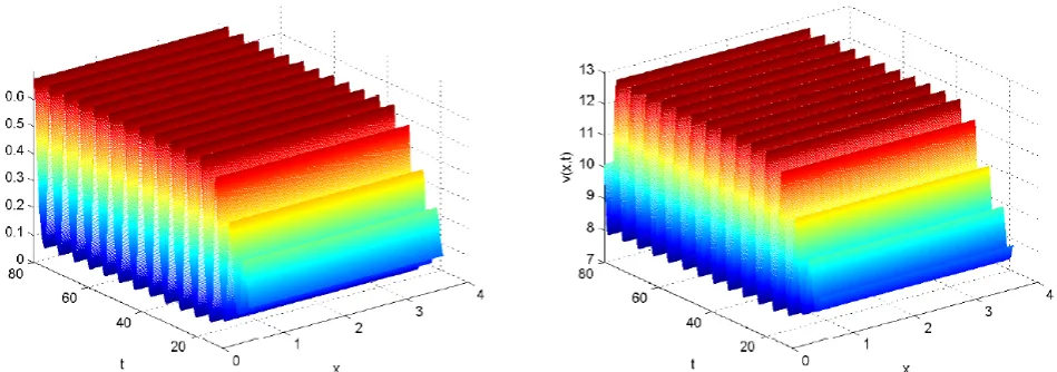
which means that Hopf bifurcation occurs only when n = 0andτ00= 0.2727.

Figure 1.Whenτ= 0.25< τ0, the positive equilibrium of system (1) is asymptotically stable with parameters given in(a), and

the initial value is(0.3,9).

Figure 2.Whenτ= 0.4> τ0, the spatial homogeneous periodic solution bifurcating from the positive equilibrium of system (1)

5. Conclusion

In this paper, we consider the diffusive Rosenzweig-MacArthur model with a constant delayτdue to the gestation of predator. We find that if condition(A)holds, then stability of the positive equilibriumE∗(u∗, v∗)was influenced by the

choose of the parameters. With the parameter set (a) as shown in section 4, we find thatE∗(u∗, v∗)loses its stability

and an spatial homogenous orbitally asymptotically stable periodic solution arises from the Hopf bifurcation when the delayτpasses through some critical valueτ0

0. This shows the

important influence of the time delayτto the system.

Acknowledgements

Thanks a lot for the kindly comments and suggestions from the reviewers and the handling editor, which led to a great improvement in the presentation of this work. In addition, this work is supported by the Doctor Foundation of Harbin University (HUDF2014-010).

References

[1] V. A. A. Jansen, The dynamics of two diffusively coupled predator-prey populations, Theoretical Population Biology, 59 (2001) 119-131.

[2] Y. Kuang, Delay differential Equation with Applications in Population Dynamics, Academic Press, New York,1993.

[3] C. S. Holling, The functional response of predator to prey density and its role in minicry and population regulation,

Mem. Ent. Sec. Can., 45 (1965) 1-60.

[4] X. Liu, L. Chen, Complex dynamics of Holling type II Lotka-Volterra predator-prey system with impulsive perturbations on the predator,Chaos, Solitons&Fractals, 16 (2003) 311-320.

[5] E. Beretta, Y. Kuang, Global analyses in some delayed ratio-dependent predator-prey systems, Nonlinear Ana. TMA., 32 (1998) 381-408.

[6] W. Ko, k. Ryu, Qualitative analysis of a predator-prey model with Holling type II functional response incorporating a prey fefuge, J. Differential Equations, 231(2006) 534-550.

[7] M. Rosinzweig and R. MacArthur, Graphical representation and stability conditions of predator-prey interation,American Naturlist, 97 (1963) 209-223.

[8] S. B. Hsu, On global stability of a predator-prey system.

Math. Biosci., 39 (1978) 1C10.

[9] S. B. Hsu, P. Waltman, Competing predators, SIAM J. Math. Anal., 35 (1978) 617-625.

[10] S. B. Hsu, T. W. Hwang and Y. Kuang,Global analysis of the Michaelis-Menten-type ratio-dependent predator-prey system.J. Math. Biol., 42 (1978) 489C506.

[11] D. Xiao, S. Ruan, Global dynamics of a ratio-dependent predator-prey system,J. Math. Biol., 43 (2001)268-290.

[12] X. Tian, R. Xu, Global dynamics of a predator-prey system with Holling type II functional response,

Nonlinear Analysis: Modelling and Control., 16 (2011) 242-253.

[13] K. Cheng, Uniqueness of a limit cycle for a predator-prey system,SIAM J. Math. Anal., 12 (1981), 541-548.

[14] Y. Kuang, H. I. Freedman, Uniqueness of limit cycles in Gause-type models of predator-prey systems,Math. Biosci., 88 (1988) 67-84.

[15] D. Xiao, Z. Zhang, On the uniqueness and nonexistence of limit cycles for predator-prey system,Nonlinearity, 16 (2003) 1-17.

[16] R. Xu, M. A. J. Chaplain, F.A. Davidson, Periodic solutons for a predator-prey model with Holling type II functional response and time delays Appl. Math. Comput., 161 (2005) 637-654.

[17] M. Banerjeea, V. Volpertbcd, Spatio-temporal pattern formation in RosenzweigCMacArthur model: Effect of nonlocal interactions,Ecological Complexity, 30(2017) 2-10.

[18] M. Moustafa, M. H.Mohd, A. I. Ismail, F, A. Abdullah, Dynamical analysis of a fractional-order RosenzweigCMacArthur model incorporating a prey refuge,Chaos, Solitons, Fractals,109,(2018) 1-13.

[19] J. Sugie, Y. Saito, Uniqueness of limit cycles in a Rosenzweig-Macarthur model with prey immigration,

SIAM J. Appl. Math., 72 (2012) 299-316.

[20] G. Zhu, J. J. Wei,Global stability and bifurcation analysis of a delayed predatorCprey system with prey immigration,Elec. J. Qual. Theo. Diff. Eqn., (2016).

[21] J. Hale, Theory of functional differential equation, Springer-Verlag, New York,1977.

[22] S. Ruan, J. Wei, On the zeros of transcentental functions with applications to stability if delay differential equations with two delays.Dyn. Contin. Discrete Impus. Syst. Ser. A Math. Anal., 10 (2003) 863-874.

[23] S. Wiggins, Introduction to applied nonlinear dynamical systems and chaos, Springer, New York, 1990.

[25] T. Faria, L. Magalh˜aes, Normal forms for retarded functional differential equations with parameters and applications to Hopf bifurcation, J. Differential Equations, 122 (1995) 181-200.

[26] J. Wu, Symmetric functional differential equations and

neural networks with memory,Trans. Am. Math. Soc., 350 (1998) 4799-838.