Volume 2010, Article ID 837237,22pages doi:10.1155/2010/837237
Research Article
Perceptually Motivated Automatic Color Contrast Enhancement
Based on Color Constancy Estimation
Anustup Choudhury and G´erard Medioni
Department of Computer Science, University of Southern California, Los Angeles, CA 90089, USA
Correspondence should be addressed to G´erard Medioni,[email protected]
Received 30 March 2010; Revised 20 August 2010; Accepted 1 October 2010
Academic Editor: Zhou Wang
Copyright © 2010 A. Choudhury and G. Medioni. This is an open access article distributed under the Creative Commons Attribution License, which permits unrestricted use, distribution, and reproduction in any medium, provided the original work is properly cited.
We address the problem of contrast enhancement for color images. Our method to enhance images is inspired from the retinex theory. We try to estimate the illumination and separate it from the reflectance component of an image. We use denoising techniques to estimate the illumination and while doing so achieve color constancy. We enhance only the illumination component of the image. The parameters for enhancement are estimated automatically. This enhanced illumination is then multiplied with the reflectance to obtain enhanced images with better contrast. We provide validation of our color constancy approach and show performance better than state-of-the-art approaches. We also show “visually better” results while comparing our enhancement results with those from other enhancement techniques and from commercial software packages. We perform statistical analysis of our results and quantitatively show that our approach produces effective image enhancement. This is validated by ratings from human observers.
1. Introduction
The human visual system (HVS) is a sophisticated mecha-nism capable of capturing a scene with very precise repre-sentation of detail and color. In the HVS, while individual sensing elements can only distinguish limited quantized levels, the entire system handles large dynamic range through various biological actions. Current capture or display devices cannot faithfully represent the entire dynamic range of the scene, therefore images taken from a camera or displayed on monitors/display devices suffer from certain limitations. As a result, bright regions of the image may appear overexposed and dark regions may appear underexposed. The objective of contrast enhancement is to improve the visual quality of images.
One of the most common techniques to enhance the contrast of images is to perform histogram equalization. The advantage of this technique is that it works very well for grayscale images; however, when histogram equalization is used to enhance color images, it may cause a shift in the color scale, resulting in artifacts and an imbalance in image color as shown inFigure 1. These unwanted artifacts are not
desirable, as it is critical to maintain the color properties of the image while enhancing them.
A high-level overview of our approach can be seen in
Figure 2. We assume any image to be a pixel-by-pixel product of the illumination (light that falls on the scene) and the reflectance component of the scene. This can be expressed as
I(x)=L(x)R(x), (1)
where L(x) is the illumination component and R(x) is the reflectance component of the image I(x) with spatial coordinatex. In this paper, we deal with color images. So,
I(x),L(x), andR(x) have 3 components—one for each color channel. For instance, for the illumination image,L(x), we denote the red color channel byLred(x), the green channel by
Lgreen(x), and the blue color channel byLblue(x). Similarly, we
(a) Original (b) Histogram Equalized
Figure1: Histogram Equalization of color images. We can see artifacts in the sky and color shift along the edges of trees.
Enhancement module
Color constancy
Remove color cast
Reflectance Illumination
Enhanced image Illumination estimation and
reflectance extraction Segment image(to remove halo
effect
Input image=illumination∗ Reflectance
Figure2: High-level overview of our method.
We first try to estimate the illumination component of the image, L(x), and thereby separate illumination from reflectance. The reason why we try to separateL(x) andR(x) is because experimentally Land [1] showed that the HVS can recognize the color in a scene irrespective of the illumination. This property of HVS is termed ascolor constancy and the theory is referred to as retinex theory. Our method also tries to mimic this human ability by removing the effects of the color of illumination from the image after estimating the illumination.
Trying to recover L(x) from an image and separate
L(x) from R(x) is a mathematically ill-posed problem, so recovering L(x) needs further assumptions. We make the assumption thatL(x) is smooth. In order to estimateL(x), based on this assumption, we smooth the image using denoising algorithms. Though this does not give us the true illumination of the scene, it gives us a good estimate of the illumination color. However, as a result of smoothing, strong halo effects can be seen along certain boundaries of the image. Therefore, before smoothing the image to estimate L(x), we preprocess the image and segment it. Smoothing can then be performed adaptively, and reduced around boundaries.
Once the color cast has been removed from the image (this is equivalent to achieving White Balance), we only process theL(x) component of the image. The motivation behind modifying only the illumination of the scene is to preserve the original properties of the scene—the reflectance of the scene. Also, the dynamic range of the illumination can be very large and hence we compress the dynamic range of the illumination. We modify the illumination of the image depending on the distribution of the intensity pixels, using logarithmic functions to estimate the enhanced illumination and then multiply it by the reflectance component to produce the enhanced image. This also helps in improving the local contrast of the image, which is another property of the human visual system. Our results show that even in complex nonuniform lighting conditions, the enhanced results look visually better.
Color constancy
Gamut-based/learning methods [3, 4, 5, 6, 7, 8]
Probabilistic methods
[9, 10]
Methods based on low level features
[1, 2, 11, 12]
Methods based on combination of methods
[13, 14, 15, 16, 17]
Figure3: Summary of previous work in color constancy.
illumination component. InSection 5, we show the results of our proposed enhancement method and compare our results with other enhancement techniques including some state-of-the-art approaches, and results from commercial image processing packages. Finally, we conclude our paper inSection 6.
2. Previous Work
2.1. Color Constancy. Most color constancy algorithms make the assumption that only one light source is used to illuminate the scene. Given the image pixel valuesI(x), the goal of color constancy is to estimate the color of light source, assuming there is a single constant source for the entire image. Alternatively, as shown in [2], the illumination is considered to be a spectrum and assuming that the color of illuminant l depends on the illuminant spectral power distributionL(λ) and camera sensitivityc(λ),lis estimated as
l=
ωL(λ)c(λ)dλ, (2)
where l is the estimated color of the illuminant, ω is the visible spectrum and λ is the wavelength. Therefore, estimatinglis equivalent to estimating its color coordinates, wherelhas 3 components—one value for each color channel. Many color constancy algorithms have been proposed to estimate the color of illumination of a scene. These methods can be broadly classified into 4 categories: (1) gamut-based/learning methods, (2) probabilistic methods, (3) methods based on low-level features, and (4) methods based on combination of different methods. The literature of these methods can be summarized as shown inFigure 3.
The gamut mapping method proposed by Forsyth [3] is based on the observation that given an illuminant, the range of RGB values present in a scene is limited. Under a known illuminant (typically, white), the set of all RGB colors is inscribed inside a convex hull and is called thecanonical gamut. This method tries to estimate the illuminant color by finding an appropriate mapping from an image gamut to the canonical gamut. Since this method could result in infeasible solutions, Finlayson et al. [4] improve the above algorithm by constraining the transformations so that the illuminant estimation corresponds to a predefined set of illuminants. Finlayson et al. [5] use the knowledge about appearance of colors under a certain illumination as a prior to estimate the probability of an illuminant from a set of illuminations. The disadvantage of this method is that the
estimation of the illuminant depends on a good model of the lights and surfaces, which is not easily available. Chakrabarti et al. [6] consider the spatial dependencies between pixels to estimate the illuminant color. Another learning-based approach by Cardei et al. [7] use a neural network to learn the illumination of a scene from a large number of training data. The disadvantage with neural networks is that the choice of training dataset heavily influences the estimation of the illuminant color. A nonparametric linear regression tool called kernel regression has also been used to estimate the illuminant chromaticity [8].
Probabilistic methods include Bayesian approaches [9] that estimate the illuminant color depending on the posterior distribution of the image data. These methods first model the relation between the illuminants and surfaces in a scene. They create a prior distribution depending on the probability of the existence of a particular illuminant or surface in a scene, and then using Bayes’s rule, compute the posterior distribution. Rosenberg et al. [10] combine the information about neighboring pixels being correlated [5] within the Bayesian framework.
A disadvantage of the above-mentioned algorithms is that they are quite complex and all the methods require large datasets of images with known values of illumination for training or as a prior. Also, the performance may be influenced by the choice of training dataset.
Another set of methods uses low level features of the image. The white-patch assumption [1] is a simple method that estimates the illuminant value by measuring the maximum value in each of the color channels. The grey-world algorithm [11] assumes that the average pixel value of a scene is grey. The grey-edge algorithm [2] measures the derivative of the image and assumes the average edge difference to be achromatic. As shown in [2], all the above low level color constancy methods can be expressed as
∂
nIσ(x)
∂xn pdx
1/ p
=kln,p,σ, (3)
where n is the order of derivative, p is the Minkowski norm andσ is the parameter for smoothing the imageI(x) with a Gaussian filter. The original formulation of (3) for the white-patch assumption and the grey-world algorithm can be found in [12]. As expressed in (3), the white-patch assumption can be expressed asl0,∞,0, the grey-world
algorithm can be expressed asl0,1,0and then-order grey-edge
(a) Original (b) Enhanced
Figure4: Halo effect caused during retinex enhancement can be observed around the edge of the body and the background.
More recent techniques to achieve color constancy use higher-level information and also use combinations of different existing color constancy methods. Reference [13] estimates the illuminant by taking a weighted average of different methods. The weights are predetermined depend-ing on the choice of dataset. Gijsenij and Gevers [14] use Weibull parameterization to get the characteristics of the image and depending on those values, divide the image space into clusters using k-means algorithm and then use the best color constancy algorithm corresponding to that cluster. The best algorithm for a cluster is learnt from the training dataset. Van de Weijer et al. [15] model an image as a combination of various semantic classes such as sky, grass, road and buildings. Depending on the likelihood of semantic content, the illuminant color is estimated corresponding to the different classes. Similarly, information about images being indoor or outdoor are also used to select a color constancy algorithm and consequently estimate the color of illuminant [16]. More recently, 3D scene geometry is used to classify images and a color constancy algorithm is chosen according to the classification results to estimate the illuminant color [17].
2.2. Enhancement Techniques. The most common technique to enhance images is to equalize the global histogram or to perform a global stretch [18]. Since this does not always gives us good results, local approaches to histogram equalization have been proposed. One such technique uses adaptive histogram equalization [18] that computes the intensity value for a pixel based on the local histogram for a local window. Another technique to obtain image enhancement is by using curvelet transformations [19]. A recent technique has been proposed by Palma-Amestoy et al. [20] that uses a variational framework based on human perception for achieving enhancement. This method also removes the color cast from the images during image enhancement unlike most
other methods and achieves the same goal as our algorithm. Inspired by the grey-world algorithm [11], Rizzi et al. [21] introduced a technique called automatic color equalization (ACE) that uses an odd function of differences between pixel intensities to enhance an image. This is a two step process— the first step computes the chromatic spatial adjustment by considering the difference in the pixels and weighted by a distance function. The second step maximizes the dynamic range of the image. A technique inspired from the retinex theory [1] is the random spray retinex (RSR) by Provenzi et al. [22] that uses local information within the retinex theory framework by replacing paths with a random 2-D pixel spray around a given pixel under consideration. The previous two techniques were fused by Provenzi et al. [23] and called RACE that account for the defects of those two algorithms (RSR has good saturation properties but cannot recover detail in dark regions whereas ACE has good detail recovery in dark regions but tends to wash out images). Another recent technique based on the retinex theory is the Kernel-based retinex (KBR) [24] that is based on computing a kernel function that represents the probability density of picking a pixel y in the neighborhood of another pixel x
removed from the reflectance component of the image using a variational approach. While enhancing the illumination channel, the technique uses only gamma-correction and the method is not automated. The user has to manually modify the value of gamma depending on the exposure conditions of the image—the value of gamma for enhancing underexposed images is very different from the value of gamma for enhancing overexposed images. A disadvantage of the techniques that are purely based on the retinex theory is that these techniques cannot enhance overexposed images because of the inherent nature of the retinex theory to always increase the pixel intensities as shown in [27]. However, this modification is tackled in both [20,24].
A recent method to obtain automated image enhance-ment is the technique proposed by Tao et al. [28] that uses an inverse sigmoid function. Due to lack of flexibility of the inverse sigmoid curve, this technique does not always result in achieving good dynamic range compression. There are other techniques that have been designed in the field of computer graphics for high dynamic range images to obtain improved color contrast enhancement. Pattanaik et al. [29] use a tone-mapping function that tries to mimic the processing of the human visual system. It applies a local filtering procedure and uses a multiscale mechanism. This technique is a local approach and it may result in halo effects. Another technique proposed by Larson et al. [30] does tone-mapping based on iterative histogram modification. Ashikhmin [31] has also proposed a tone-mapping algorithm for enhancement and is based on a Gaussian pyramid framework.
3. Our Approach to Achieve Color Constancy
As stated earlier, color constancy is the human ability to perceive the color of a scene irrespective of the illumination conditions. Therefore, to achieve color constancy, we should estimate the color of illumination. In order to estimate the color of the illumination of an image, we first process the image to estimate the illumination component, L(x). We make the assumption that L(x) is smooth. Based on this assumption, we use denoising techniques to process the image and smooth it. Denoising techniques are traditionally used in image processing to remove noise from the image. This involves smoothing of the images and hence removal of the noise. Because of our smoothness assumption ofL(x), the smooth image that is obtained by denoising, is our estimate of the illumination image, L(x). Once we have estimated
L(x), we apply the white-patch Assumption (maximum in each color channel), as described inSection 3.2onL(x) to estimate the color of the illumination.
In the most simple filtering example, the smoothing operation calculates the average of a region around every pixel of the image. As the size of the region increases (limited by the size of the image), the estimate of the maximum value in each color channel tends towards the average value in each color channel. Therefore, in a way that Minkowski norm works as mentioned in Section 2, the smoothing operation unifies the White Patch Assumption [1] and the
grey-world algorithm [11] in one approach. Hence, similar to (3), we also assume the true color of illumination to be somewhere between the maximum and the mean of the color channels. These trends in the estimate of the illumination color while filtering using different parameters are explained inSection 3.3.2.
3.1. Denoising Techniques. We study 4 different existing denoising techniques to smooth the image: (1) Gaussian filter, (2) median filter, (3) bilateral filter, and (4) nonLocal means filter. These filters have different levels of complexity and vary in their smoothness mechanism. We consider the input imageI(x) to be defined on a bounded domainΩ⊂R2
and letx∈Ω. The description of these filters is given below.
3.1.1. Gaussian Filter. Blurring the image removes noise. This filter can be expressed as
G(x)= 1
2πσ2e
(−|x|2/2σ2)
, (4)
whereσ is the smoothing parameter. This is a 2D Gaussian radially symmetric kernel where|x| =(x2+y2)1/2
.
Gijsenij and Gevers [32] have explored iterated local averaging and can be considered similar to the Gaussian filter approach. The edge information is lost during Gaussian filter and this introduces error while estimating the illuminant. We apply this filter across all 3 color channels (red, green and blue) of the image.
3.1.2. Median Filter. For every pixel in an image, the median filter [33] chooses the median color value amongst the neighborhood pixels in a windowW for that pixel—every pixel has same number of color values above and below it. Smoothing using median filter may result in the loss of fine details of the image though boundaries may be preserved. We apply this filter on all 3 color channels (red, green and blue) of the image.
3.1.3. Bilateral Filter. In case of bilateral filter [34], every pixel of the image is replaced by a weighted sum of its neighbors. The neighboring pixels are chosen from a window (W) around a given pixel. The weights depend on two parameters: (1) Proximity of the neighboring pixels to the current pixel (Closeness function) and (2) similarity of the neighboring pixels to the current pixel (similarity function). The closer and the more similar pixels are given higher weights. The two parameters can be combined to describe the bilateral filter as follows:
L(x)=k−1(x)
W(x)c
y,xsIy,I(x)Iydy, (5)
whereyis the neighboring pixel and the normalization term
kcan be given by:
k(x)=
W(x)c
y,xsIy,I(x)dy. (6)
The closeness function is
whered(y,x)= y−xis the Euclidean distance between a given pixel,xand its neighbory. The similarity function is
sIy,I(x)=e−(1/2)(δ(I(y),I(x))/σs)2, (8)
whereδ(I(y),I(x)) is the pixel value difference betweenxand
y. The closeness function from (7) having standard deviation
σc and the similarity function from (8) having standard deviationσsare Gaussian functions of the Euclidean distance between their parameters. In the original implementation of the bilateral filter, Tomasi and Manduchi [34] have used the CIELAB color space. We present results by applying this filter on all 3 channels of the CIELAB color space of the image. Applying this filter on the RGB colorspace instead does not result in a significant difference.
3.1.4. Nonlocal Means Filter. The hypothesis behind nonlocal means (NL-means) technique [35] is that for any image, the most similar pixels to a given pixel need not be close to it. They could lie anywhere in the image. For comparing how similar the pixels are, instead of checking the difference between the pixel values (which is used in bilateral filtering), the neighborhood of the pixel is considered—that is, comparison of a window around the pixel is done. This technique uses self-similarity in an image to reduce the noise. The formulation of the NL-means filter is:
NL(I(x))=L(x)
= 1
N(x)
Ωe
−(Gρ∗|I(x+·)−I(y+·)|2)(0)/h2Iydy,
(9)
where y ∈ Ω, I(x) is the observed intensity at pixel x,
Gρ is a Gaussian kernel with standard deviationρ,his the filtering parameter that controls the amount of smoothing andN(x) is the normalizing factor. Equation (9) means that an image pixel valueI(x) is replaced by the weighted average of other pixel values in the image I(y). The weights are significant only if a window around pixel x looks like the corresponding window around pixely. While comparing the windows, we consider the Euclidean distance between the 2 windows. However, we weigh this distance by a Gaussian-like kernel decaying from the center of the window to its boundaries. This is because closer pixels are more related, and so pixels closer to the reference pixel are given more importance. Ideally, we should search the entire image to find a similar neighborhood. But for efficient computation, we consider a smaller local search area,S. The numerator of the exponential accounts for the neighborhood of a pixel which we denote by W. Please refer to [35] for a more detailed explanation of the NL-means filter. For discrete images, the integral overΩcan be replaced by a summation over all pixels of the image. We apply this filter on all 3 color channels (red, green and blue) of the image.
3.2. Illuminant Color Estimation. Once we have obtained the illumination image L(x), by smoothing the original color image I(x), in order to estimate the color of the illuminationl, we use the white-patch assumption [1]. This method computes the maximum values of each of the 3 color
channels—red, green and blue. The proposed formulation forlis
l=
max
x
Lred(x)
, max
x Lgreen(x)
, max x
Lblue(x)
, (10)
whereLred(x),Lgreen(x) andLblue(x) are the red, green, and
blue color channels of the denoised image (illumination image) and the max operation is performed on the separate color channels. The maximum value of these color channels need not lie at the same pixel of the image. This estimation is based on the hypothesis that since a white patch of the image reflects all the light that is incident on it, its position can be found by searching for the maximum values of the red, green and blue channels. Thelvector thus estimated is normalized and is denoted byl, which has 3 components:l(1),l(2) and l(3) for red, green, and blue respectively.
Once the color of the illumination is estimated as described above, we remove the effect of color cast from the image. This is equivalent to adding white light to the scene. This can be represented as
Lredcolor-corrected(x)= 1
√
3
Lred(x)
l(1) ,
Lgreencolor-corrected(x)= 1
√
3
Lgreen(x)
l(2) ,
Lbluecolor-corrected(x)= 1
√
3
Lblue(x)
l(3) ,
(11)
where the factor√3 is the normalization constant based on the diagonal model to preserve the intensity of pixels. Com-bining all 3 color channels—Lredcolor-corrected(x),Lgreencolor-corrected(x) and Lbluecolor-corrected(x), shown in (11)—gives us the color corrected image. This is how we obtain the images illustrated inFigure 12.
3.3. Evaluation and Discussion. In order to evaluate our approach, we conduct experiments on two widely used datasets. The ground-truth values of the illuminant of the scenes are provided for both datasets. For quantitative evaluation of the approaches, the error difference between the estimated illumination color l and the ground truth illumination colorlgtis computed. We use the angular error
as a measure and it can be computed as
angular error, =cos−1 l·lgt
, (12)
where (·) stands for normalized values. In order to measure the overall performance across each of the datasets, the median of the angular errors is considered as a suitable measure [36].
(a) (b) (c) Figure5: Images from the controlled indoor environment [37].
Table1: Error for the controlled indoor environment using various color constancy methods. The parameters of our approach have been described inSection 3.1. The best result is reported in bold.
Method Parameters Median(◦) RMSrg
White-patch — 6.4 0.053
Grey-world — 6.9 —
1st-order grey edge p=7 3.2 —
2nd-order grey edge p=7 2.8 —
Color by correlation — 3.1 0.061
Gamut mapping — 2.9 —
Neural networks — 7.7 0.071
GCIE version 3, 11 lights — 1.3 —
GCIE version 3, 87 lights — 2.6 —
Kernel regression — — 0.052
Support vector machines — — 0.066
Gaussian filter σ=3,x=30 2.9 0.043
Median filter W=20 2.4 0.044
Bilateral filter σc=2,σs=5,W=5 2.8 0.044
NL-means filter h=0.2,S=3,W=2 2.5 0.043
by the original authors and therefore, this dataset has 321 images. Some sample images from this dataset can be seen inFigure 5. All images have resolution of 637×468 pixels.
The results of existing color constancy algorithms on this dataset are summarized inTable 1. These results are available in [2,4,36]. Some methods in the literature [8] have used the root mean square (RMS) error between the estimated illuminantion chromaticity,lce and the actual illumination chromaticity, lcgt to evaluate their results although this is
not the best metric [36]. Since we do not have access to the individual error values, we compare the results as is. The RMSrgerror can be calculated as
RMSrg=
⎛ ⎝1
N N
i=1
1
M M
j=1
lci
j−lcgti
j2
⎞ ⎠
1/2
, (13)
where N is the total number of images, i is the index of images and M is the number of color channels (M = 2 for chromaticity space). We calculate error for the rg space. The chromaticity for r andg for the estimated illuminant can be computed as lc(1) = l(1)/(l(1) +l(2) +l(3)) and
lc(2) =l(2)/(l(1) +l(2) +l(3)). Similarly, we can compute
the chromaticity for the ground truth illuminant. The RMSrgerror for white-patch, Neural Networks and Color by
Correlation were presented in [38]. The performance of our approach on this dataset are also presented inTable 1.
From Table 1, we can see that our approach gives the best performance both with respect to the angular error and the RMSrgerror. On comparing the error of our approach
with that of all the approaches in [38], we can see that our approach has the least RMSrg error. The GCIE algorithm
using 11 lights perform very well because this technique uses the 11 illuminants as a prior knowledge. It constrains the estimated value of the illuminant to lie in that set. However, the performace drops if more illuminants are used for training. We also compared our results with a recent denoising technique by Dabov et al. [39]. However, their technique produces a median error of 5.67◦on this dataset which is worse than our results.
0 10 20 30 40 50 60 0
10 20
30 40
−4.5
−4
−3.5
−3
−2.5
σ Kernel
siz e
M
edian
angular
er
ror
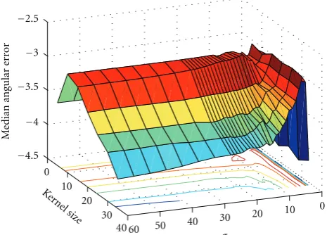
Figure6: Median angular error as a function ofσand kernel size for a Gaussian filter.
The axis for the median angular error is inverted for better visualization.
The error plot for Gaussian filter is shown inFigure 6. Smoothing withσ =0 will have no effect and therefore, for
σ =0, this method works like the white-patch assumption. However, asσ → ∞, the algorithm is equivalent to taking the average of the image and therefore, the algorithm is equivalent to the grey-world algorithm. We obtain the best results for an intermediate value of σ. Also from the plot, we can see that for lower values of σ, the median angular error remains fairly consistent for higher values of window size. This is because in case of a Gaussian distribution, 99.7% pixels values lie within 3σof the mean and therefore higher values of window size does not affect the calculation of a pixel value. Also, for higher values ofσ, we can see that the error value increases with increase in window size. Irrespective of the σ values, typically window size of around 5–20 pixels gives us best results.
The error plot for median filter is shown inFigure 7. As can be seen in the case of Gaussian filter, we can see that we obtain best error values for window size (W) of around 5–20 pixels. ForW =0, this algorithm is once again the same as white-patch algorithm. However when the value ofW → ∞, the color estimated by this method will be the median color value of all the pixels present in the image. Realistically, the limiting factor forWwill be the image size. For this dataset, the median angular error whenWis the image size, is12.99◦. The error plot for Nonlocal means filter is shown in
Figure 8. In case of a Nonlocal means filter, the amount of smoothing of the image depends on the filtering parameter,
h. A higher value ofhdoes more smoothing of the image. As we can see inFigure 8, the error value converges for higher values ofh. Forh= 0, the algorithm will not perform any smoothing and this method will be the same as the white-patch algorithm.
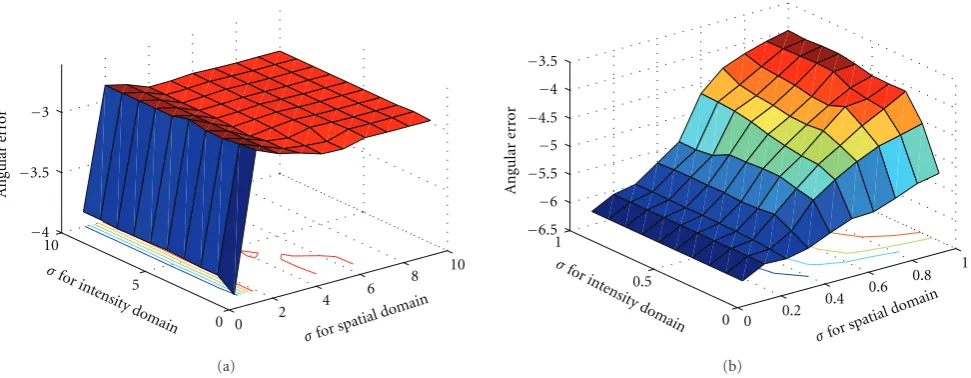
The error plots for bilateral filter are shown in Figures9
and10. The left image ofFigure 9plots the median angular error for low values of σ for spatial domain, σc and σ for intensity domain, σs whereas the right image plots the
0 5 10 15 20 25 30 35
−6.5
−6
−5.5
−5
−4.5
−4
−3.5
−3
−2.5
−2
Window size
M
edian
angular
er
ro
r
Figure7: Median angular error as a function of window size for a median filter.
10−3 10−2 10−1 100 101
−5.5
−5
−4.5
−4
−3.5
−3
−2.5
Filtering parameter (h)
M
edian
angular
er
ror
Figure8: Median angular error as a function of filtering parameter for a Nonlocal means filter.
median angular error for high values ofσc andσs. As with the Nonlocal means filter, we can see that the error value converges for high smoothing (high values of σc and σs). For values of σ’s = 0, this algorithm will behave like the White Patch algorithm. The best results are obtained from an intermediate value of smoothing parameter.
As shown inFigure 10, given the best values ofσcandσs, we see the effects of changing the window size on the median errors. For low window size, since there is not enough information, the error values are high. However, since the individual closeness and similarity functions are Gaussian distributions, having a very high window size does not help much and the error value converges close to the best value.
0 2
4 6
8 10
0 5
10
−4
−3.5
−3
σfor spatial domain σfor
intensit y domain
A
n
gular
er
ror
(a)
0 0.2
0.4 0.6
0.8 1
0 0.5
1
−6.5
−6
−5.5
−5
−4.5
−4
−3.5
σforspat ial doma
in σfor int
ensit y domai
n
A
n
gular
er
ro
r
(b) Figure9: Median angular error as a function ofσ’s for a bilateral filter.
0 5 10 15 20 25 30
−4.2
−4
−3.8
−3.6
−3.4
−3.2
−3
−2.8
−2.6
Window size
A
n
gular
er
ro
r
Figure10: Median angular error as a function of window size for a bilateral filter.
images from this dataset can be seen inFigure 11. The images include both indoor and outdoor scenes. All images have 360×240 resolution as they are all extracted from a digital video. As a result, there is a high correlation between the images from one scene in the database. Therefore, from each scene we randomly select 10 images amounting to 150 images in total on which we test our approach. Some sample images from this dataset can be seen inFigure 11.
As can be seen in Figure 11, all the images from this dataset have a grey ball at the bottom right corner of the image. This grey ball was mounted on the video camera to estimate the ground truth value of the color of the illuminant and those values are available with the dataset. However, while trying to estimate the illuminant color, we exclude the bottom right quadrant as depicted by the white box in
Figure 12.
The results of existing color constancy algorithms and our approaches on this dataset can be found in Table 2. The selection of parameters significantly improves the results when compared with the state-of-the-art color constancy approaches. From Table 2, we can see that our method have a23% improvement over the state-of-the-art grey-edge algorithm. We also compared our algorithm with a very recent technique—“Beyond Bag of pixels” approach [6] and found that our method gives us almost26% improvement. On comparing our results with a recent denoising technique by Dabov et al. [39], that produces a median error of 3.96◦, we obtain an improvement of almost14%.
3.3.4. Discussion. From the experiments that we have con-ducted on the 2 widely used datasets and the results pre-sented in Tables1and2, we can see that our approach gives us results that are better than state-of-the-art color constancy approaches. On the controlled indoor environment dataset, [2] have reported a median error of 3.2◦ for the 1st order grey-edge algorithm with p = 7 and preprocessing with a Gaussian filter of σ = 4. The median error for the same dataset for the 2nd order grey-edge algorithm with p = 7 and preprocessing with a Gaussian filter ofσ =5 is 2.7◦. Our experiments have shown that using just a Gaussian filter with
σ =4 gives us a median error of 3.08◦and withσ =5 gives us a median error of 3.12◦. This makes us wonder if applying 1st order grey-edge algorithm hurts the illuminant color estimation. However there are benefits of using higher order grey-edge color constancy algorithms. It will be interesting to explore how grey-edge color constancy algorithms with ordern >2 affect the estimation of illuminant color. It will also be interesting to observe how complex methods such as GCIE, neural networks and other learning methods perform on images that are already preprocessed by our approach.
(a) (b) (c) Figure11: Images from the real-world environment [40].
Table2: Median angular error for the real-world environment. The parameters of our approach have been described inSection 3.1. The best result is reported in bold.
Method Parameters Median(◦)
White-patch — 4.85
Grey world — 7.36
1st-order grey edge p=6 4.41
Beyond bags of pixels — 4.58
Gaussian filter σ=5,x=15 3.63
Median filter W=9 3.42
Bilateral filter σc=5,σs=7,W=3 3.4 NL-means filter h=1.0,S=3,W=2 3.39
Table3: Ranks of algorithm according to Wilcoxon signed rank Test. The best results are reported in bold.
Method WSTs
White-patch 1
Grey world 0
1st-order grey edge 2
Gaussian filter 2
Median filter 2
Bilateral filter 3
NL-means filter 3
dataset. This could be because the controlled environment dataset does not have too much variability—it consists of an object or two with/without a background. However, for the real-world dataset, there is a lot of variability and so more information is available even in a small window.
As shown in [35], amongst the filters described here, NL-means filter performs the best denoising. It best preserves the structure of the image while denoising the image. We observe a similar correspondence between the denoising capabilities of the filter and its illumination color estimation. The best illumination estimation results are obtained by using the best denoising filters.
In order to compare the performance of different color constancy algorithms, we use the Wilcoxon signed-rank test [41]. For a given dataset (We choose the real-world environment dataset), let C1 and C2 denote the angular
error between the illuminant estimation of two different
algorithms and the ground truth illuminant values. Let the medians of these 2 angular errors be mc1 and mc2. The Wilcoxon signed-rank test is used to test the null hypothesis
H0 :mc1 =mc2. In order to test this hypothesis, for each of Nimages, the angular error difference is considered—(e1
c1− e1
c2), (e2c1−e2c2),. . ., (eNc1 −eNc2). These error pairs are ranked according to their absolute differences. If the hypothesisH0
is correct, the sum of the ranks is 0. However, if the sum of ranks is different from 0, we consider the alternate hypothesis
H1 : mc1 < mc2 to be true. We reject/accept the hypothesis if the probability of observing the error differences is less than or equal to a given significance level α. We compare every color constancy algorithm with every other color constancy algorithm and generate a score that tells us the number of times a given algorithm has been considered to be significantlybetter than the others. The results are presented inTable 3.
4. Our Image Enhancement Method
Our method for image enhancement is motivated by illuminance-reflectance modeling. It consists of 2 key steps: (1) Illumination estimation using Nonlocal means technique (2) Automatic enhancement of illumination. The flowchart of our enhancement module is shown inFigure 13. For our illumination estimation, we use the Nonlocal means(NL-means) technique because as shown in Section 3.3.3, it performs amongst the best while trying to estimate the color of illumination. Also as shown in [35], NL-means filter does a very good job at preserving the original structure of the image while smoothing the image.
Original images
Correction using ground truth values
Correction using white patch assumption
Correction using grey world algorithm
Correction using grey edge algorithm
Correction using Gaussian filter
Correction using median filter
4.71◦ 4.82◦ 3.24◦ 6.45◦
7.17◦ 22.14◦ 13.28◦ 8.37◦
8.09◦ 6.26◦ 1.03◦ 3.26◦
1.98◦ 3.59◦ 4.50◦ 0.95◦
0.93◦ 0.80◦ 1.53◦ 0.88◦
2.01◦ 1.12◦ 2.74◦ 0.73◦
0.93◦ 0.78◦ 1.43◦ 0.51◦
Correction using bilateral filter
Correction using non-local means filter
Enhancement module
Enhanced luminance Luminance
Chrominance Split into luminance
and chrominance Reflectance
Color-cast removed illumination
Enhanced image Combine luminance
and chrominance Automatic
enhancement using
mapping function Enhanced
illumination
Figure13: Flowchart of the enhancement module.
multiplying it back with the reflectance causes strong halo effects. In order to remove the halo effect, we presegment the image using Mean-shift segmentation algorithm proposed by Comaniciu and Meer [42]. Any segmentation algorithm can be used. The boundaries of the segmented image is used as a preliminary information for the smoothing process. While trying to estimate the illumination, when we consider a neighborhood for every pixel, we also consider the same spatial neighborhood of the presegmented image and if an edge occurs in the presegmented image, less smoothing is done (h = 0.01). This helps in preserving high contrast boundaries of the image and thus removes the halo effect from the image.
Once the illumination componentL(x) has been esti-mated, the reflectance component of the image R(x) for every pixel x can be calculated as the pixel-by-pixel ratio of the image and the illumination component and can be expressed as
R(x)= I(x)
L(x), (14)
where I(x) is the original image. Alternatively, in the logarithm domain, the difference betweenI(x) andL(x) can be used to estimateR(x).
As shown inSection 3.2, once we estimate the color of illumination, we remove the effect of color cast fromL(x). We first estimate the color of illumination as shown in (10). Then as shown in (11), we remove the effect of color cast from each of the 3 color channels (red, green and blue) and then combine all 3 new color channels to get color-corrected illumination image,Lcc(x).
4.2. Automatic Enhancement of Illumination. In order to preserve the color properties of the image, we modify only the brightness component of the image. The illumination
Lcc(x) obtained from Section 4.1 is converted from RGB color space to HSV color space and only the luminance (V) channel—LccV(x) is modified. Alternatively, CIELAB
color space could be used and modification of the lightness channel can be done. The chrominance channels are not modified to preserve the color properties of the image.
0 0.2 0.4 0.6 0.8 1
0 0.1 0.2 0.3 0.4 0.5 0.6 0.7 0.8 0.9 1
Input intensity
Enhanc
ed
Int
ensit
y
Bright region→
←x=0.6 controlPt
←Dark region
Figure14: The mapping function for enhancement.
Our method can be used for images that are underex-posed, overexposed or a combination of both. Since, we have to deal with different exposure conditions, our enhancement method deals with those cases separately and divide the intensity of the illumination map into 2 different regions as shown inFigure 14.
The division of the region is determined by the position-ing of the controlPt. The value of controlPtis computed as follows:
controlPt=
LccV(x)≤0.51
LccV(x)≤11
. (15)
Intuitively, if an image is heavily underexposed, then a lot of pixels will have very low intensity values. Using (15) we can see that, for such images, the value of controlPt → 1. Similarly, if an image is heavily overexposed, then a lot of pixels will have very high intensity values causing the value of controlPt → 0. Thus, we can see that the controlPt∈[0.5, 1] for images that are predominantly underexposed whereas controlPt∈[0, 0.5] for predominantly overexposed images.
For underexposed regions,
Choose blue curve dark=
LccV(x)≤0.11
LccV(x)≤11 > T1
Choose green curve Otherwise.
(16)
If a lot of pixels lie in the dark region, then we have to enhance the values of those pixels by a larger value. As a result, the blue curve will be chosen. Otherwise, we will choose the green curve to enhance the pixels that lie in (0.1, controlPt] region.
For overexposed regions,
Choose green curve bright=
LccV(x)≥0.91
LccV(x)≤11 > T2
Choose blue curve Otherwise.
(17)
Similarly, if a lot of pixels lie in the bright region, then we have to reduce the values of those pixels by a larger value. Therefore, we will choose the green curve. Otherwise, in order to enhance the pixels that lie in (controlPt, 0.9), we choose the blue curve.
The thresholdsT1=0.01 andT2=0.01 are determined
experimentally and those values were chosen that gave the best enhancement results over a wide range of images.
The curves are represented as a logarithmic function. The blue curve can be represented as
LenhV(x)=v1+
1
Klog
LccV(x)−v1
ρ+ 1(v2−v1), (18)
and the green curve can be represented as
LenhV(x)=v2−
1
K log
v2−LccV(x)
ρ+ 1(v2−v1). (19)
where K = log(ρ(v2 − v1) + 1 is a constant and
LccV(x) ∈ [v1,v2]. For underexposed regions of the image, LccV(x) ∈ [0, controlPt] and for overexposed regions, LccV(x) ∈ (controlPt, 1]. The formulation of the curves in
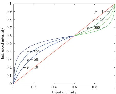
(18) and (19) is inspired by the Weber-Fechner law that states that the relationship between the physical magnitude of the stimuli and the perceived intensity of the stimuli is logarithmic. This relationship was also explored by Stock-ham [43] and Drago et al. [44] who also recommended a similar logarithmic relationship for tone mapping purposes. Our formulation, inspired by the HVS, is different in flavor from the existing formulations. It takes care of the diff er-ent exposure conditions simultaneously and automatically estimates the parameters across a wide variety of images, thus enhancing those images without additonal manual intervention.
ρ represents the curvature of the curve, and enhances the intensity of illumination accordingly. For instance, in an underexposed region, due to higher value of dark, the intensity has to be increased more and so a higher value ofρ
is used for the first curve. Similarly in an overexposed region, due to higher value of bright, we decrease the intensity of those regions by a higher value and therefore, a higher value
0 0.2 0.4 0.6 0.8 1
0 0.1 0.2 0.3 0.4 0.5 0.6 0.7 0.8 0.9 1
←ρ=50
←ρ=500
←ρ=10
ρ=500→
ρ=50→
ρ=10→
Input intensity Enhanc ed int ensit y
Figure15: The effects of changing the value ofρ.
ofρis used for the second curve. This effect is depicted in
Figure 15.
LenhV(x) is the enhanced luminance. This is combined
with the original chrominance to obtain the enhanced illumination—Lenh(x).
4.3. Combining Enhanced Illumination with Reflectance. The enhanced illumination, Lenh(x) that was obtained in
Section 4.2 is multiplied with the reflectance component
R(x) that was obtained in Section 4.1 to produce the enhanced imageIenh(x) as follows:
Ienh(x)=Lenh(x)R(x), (20)
The entire process is automated and the enhancement occurs depending on the distribution of the pixels in the image.
5. Results and Discussion
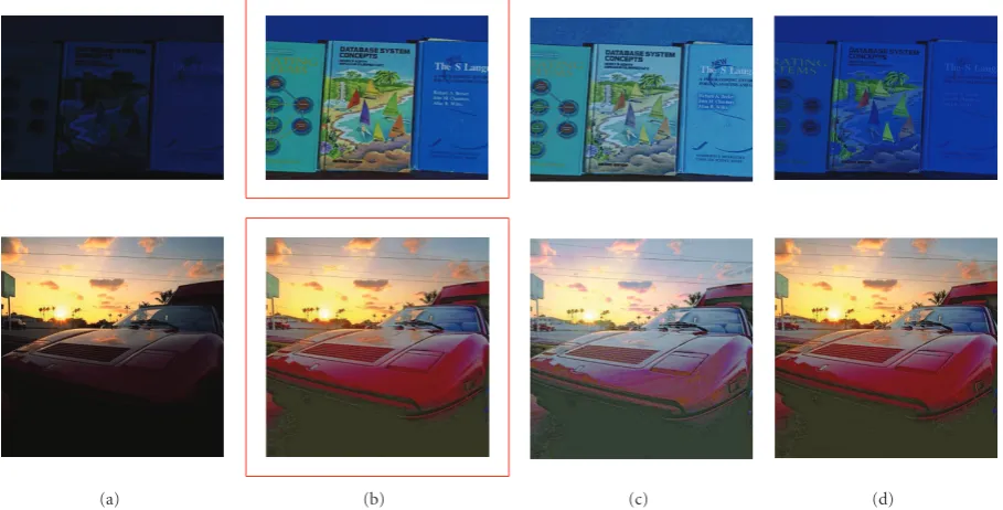
(a) (b) (c) (d)
Figure16: Enhancement according to our algorithm. Column (a) is the original images. Column (b) is enhancements according to our implementation. Column (c) is enhancements on all 3 color channels of the illumination. Column (d) is enhancements on the intensity channel of the illumination.
Finally, we perform statistical analysis and quantitative evaluation followed by human validation to demonstrate the effectiveness of our enhancement algorithm.
5.1. Computational Cost. We have implemented the algo-rithm in MATLAB in Windows XP environment on a PC with Xeon processor. For an image with size 360 ×240 pixels, segmentation takes 6 sec., illumination estimation takes 39 sec. and the enhancement of illumination takes
<1 sec. The speed can be improved by implementing the code in C++. Also, faster and more optimized versions of NL means filter can be used to increase the computational efficiency.
5.2. Enhancement Results. In order to display the results of our enhancement, we consider two different images as shown in Figure 16(a). The top image, obtained from the database provided by Barnard et al. [37], is taken under strong blue illumination while the bottom image is obtained courtesy of P. Greenspun (http://philip.greenspun.com/), and is underexposed.
The results of our algorithm is presented inFigure 16(b). The contrast of the enhanced images is much better than the original images and the color cast from the images has also been removed. For comparison, enhancement was done on all 3 color channels of the original illuminationL(x) as shown inFigure 16(c). It helped in removing the color cast but also resulted in a loss of color from the original image. Enhancement was also done on only the intensity channel of the original illuminationL(x) as shown inFigure 16(d)and it did not help in removing the color cast as shown in the top image. Therefore, our technique produces the best of both
worlds—it enhances the color of the scene as well as it helps in removing the color cast from the image. Further, it also gives us a visually pleasant image.
5.3. Comparison with Other Methods. We have also com-pared our results with existing methods such as histogram equalization. Histogram equalization on all 3 color channels of the original image results in color shift and loss of color as shown inFigure 17. It also results in artifacts. The histogram equalization on only the luminance channel as shown inFigure 18does not result in color shift but it also does not improve the visual quality of images with color cast.
We have compared with the variational approach in retinex proposed by Kimmel et al. [26] and have used our implementation of the proposed technique. This tech-nique uses gamma correction to modify the illumination. The method is not automated and the value of gamma required for enhancing the images depends on the quality of the original images (underexposed/overexposed) and it is cumbersome to manually adjust it. The output from this technique is shown in Figure 19. When we compare this to the output that we get as shown on the top image in
Figure 16(b), we can see that our method produces better enhancement.
(a) (b)
Figure17: Histogram equalization on all 3 color channels of the input image. Color shifts and artifacts are quite prominent.
(a) (b)
Figure18: Histogram equalization on the luminance channel of the input image. Color cast persists and does not improve the contrast of image.
(a) (b)
(a)
(b) (c)
Figure20: (a) is the original image. (b) is enhanced by McCann retinex and (c) is enhanced by our algorithm. More detail can be seen in the shadows and no halo effect exists in our implementation.
We have also compared our results with a recent tech-niques proposed by Palma-Amestoy et al. [20] and Provenzi et al. [21–23],and observe that our methods give better contrast and the resulting images look visually better as shown inFigure 21.
We also compared our results with the MSRCR algorithm and observed that our results have a better contrast than the output of the PhotoFlair software as shown inFigure 22. The original images and the output of MSRCR were obtained from NASA website (http://dragon.larc.nasa.gov/ retinex/pao/news).
Finally, we compared our algorithm with the output given by Picasa. We used theAuto Contrastfeature of Picasa and as shown inFigure 23, we can see that we obtain better results. Other parameters can be manually modified in Picasa to get better results but we are building an automated system with no manual tuning of parameters. Even in our approach, if necessary, we can also manually modify parameters to obtain different looking results.
We also compared our algorithm with the output given by DXO Optics Pro and the results are shown inFigure 24.
5.4. Statistical Analysis. A good way to compare an image enhancement algorithm is to measure the change in image quality in terms of brightness and contrast [28]. For measuring the brightness of the image, the mean brightness of the image is considered and for measuring the contrast of the image, local standard deviation of the image (standard deviation of image blocks) is considered. In Figure 25, the mean brightness and local standard deviation of the image blocks for the top image ofFigure 16(a)(size of image block is 50×50 pixels) is plotted before and after enhancement. We can see that there is a marked difference (increase) in both the brightness and the local contrast after image enhancement.
5.5. Quantitative Evaluation. A quantitative method to eval-uate enhancement algorithms depending on visual repre-sentation was devised by Jobson et al. [46] where a region of 2D space of mean of the image and local standard deviation of the image was defined asvisually optimal, after testing it on a large number of images. We have shown the effects of implementing our algorithm inFigure 26. It can be seen that some of the enhanced images (overexposed and underexposed before enhancement) lie inside the visually optimal region whereas other images though do not lie in thevisually optimalregion have a tendency to move towards that region. This happens because those original images are either too dark (very underexposed) or too bright (very overexposed).
We also visualize the effects of other enhancement algo-rithms inFigure 26. We observe that more images enhanced by our method lie closer/in thevisually optimalregion than the images enhanced by MSRCR. For images that are heavily overexposed, we can see that our enhancements lie closer to the visually optimal region than the ones enhanced by Picasa. Some images, for instance, image with μμ ≈ 42 and μσ ≈ 5 are enhanced by multiple methods and we can see that our enhanced images lie closer to thevisually optimalregion than the other enhancement methods. On an average, our approach results in “better” enhancement than existing techniques. However, “better” enhancement is very subjective so we conduct human validation of our approach, as described inSection 5.6.
Some interesting observations are as follows—Histogram Equalization (both on 3 color channels or the intensity channel) results in the enhanced image being in thevisually optimalregion whereas our enhanced image lies very close to that region. This is because as can be seen inFigure 17
(a) (b) (c)
(d) (e)
Figure21: (a), (b), and (c): Enhancements by Rizzi et al. and Provenzi et al. (a) is enhanced by RSR [22], (b) is enhanced by ACE [21] and (c) is enhanced by RACE [23]. The images are obtained from [23]. (d) and (e): (d) is obtained from [20] whereas (e) is using our algorithm. Note the color contrast amongst the images. Also on zooming in the image, theprancing horsecan be seen more clearly on (e).
increase the local standard deviation thus causing an increase in the value ofμσresulting in the histogram equalized image to lie in thevisually optimalregion. Also for an image that already lies in thevisually optimalregion, we can see that our enhancement does not result in a significant change. In short, our enhancement does not spoil the visual quality of good quality images. This has also been validated by experiments on human observers as shown inSection 5.6.
5.6. Human Validation. To know the effectiveness of our method, we enhanced 40 images using our algorithm. The procedure has 2 steps: (1) We presented the original and the enhanced version simultaneously. The placement of the original and the enhanced version were random(either the left or the right side of the screen) to remove any bias that may exist while selecting an image. We asked each of the 12 human observers independently to rate the image on the “right” side as “better”, “same” or “worse” relative to the image on “left” side of the screen and recorded their responses. Scores were thus assigned as 1 for Better, 0 for Sameand −1 for Worse. These responses were used to evaluate the “preference” for enhanced image. (2) The original image was then presented on the screen and the observers were asked to rate the “quality” of the image as
“poor”, “average” or “good” that was recorded as 1, 2 or 3 respectively. The people were unaware of the fact that the image in Step 2 that is being presented to them is the original image from Step 1 to remove any bias that may occur due to knowledge of the original image.
This was repeated for all 40 images in the database. Finally, one image that had the most perceptible difference after enhancement was presented to the subject but with the order flipped from the previous display and the response was noted to check if the subjects were consistent with their responses.
We found that observers were not biased towards select-ing any one side of the screen. The responses of all the subjects were also consistent when the “preference” ratings for the last comparison was compared with that of its earlier ratings.
Figure 27shows the original image “quality” ratings. We can see that around 72.5% of images were ratedabove Average (quality>=2) by people.
Similarly,Figure 28shows the “preference” ratings for the enhancement method. We can see that in most cases, the observers prefer our enhanced images.
(a)
(b)
(c)
Figure22: (a) is the original images. (b) is the enhanced images by MSRCR. (c) is the images enhanced by our algorithm. Using our algorithm, we can clearly see the red brick wall within the pillars on the left image and some colored texture on the white part of the shoe can be clearly seen.
quality of those original images (Figure 27), we can see that 3 of those images were rated high (quality>2.5). Also for all the 4 cases where enhanced images were considered to be the same as the original images (preference=0), the quality of the original images was rated was rated high (quality>2.5). For all the cases where the original images were ratedPoor (quality=1), the observers consistently showed preference for the enhanced images (preference>0).
Further, using Wilcoxon signed-rank test [41], we inferred that the enhanced images are statistically signifi-cantly differentfrom the original image (The null hypothesis of zero median of the difference is rejected at 5% level) and by comparing the ranks we conclude that the enhanced images have a higher rank than the original images. This implies that people prefer enhanced images over the original images.
6. Conclusion
(a) (b)
Figure23: (a) is the enhanced output usingAuto Contrastfeature of Picasa and (b) is enhanced using our algorithm.
(a) (b)
Figure24: (a) is enhanced using DXO Optics Pro and (b) enhanced using our algorithm.
parameters to tune them and adjust the values according to their needs to get customized enhancements. Our method also does not suffer from halo effects during enhancement nor does it suffer from any color shifts or color artifacts or noise magnification. Experimentally, we have compared our enhancement results with results from other existing
10 20 30 40 50 60 0 50 100 0 50 100 M ean of image Image blocks Local standar d d ev iation Original mean Original STD Enhanced mean Enhanced STD
Figure25: Statistical characteristics of the image before and after enhancement. 20 40 60 80 100 120 140 160 180 200
Mean of standard deviation (μσ) Visually optimal
Original image Our enhancement Picasa
MSRCR
Hist. equalizn. (color) Hist. equalizn. (intensity) Kimmel’s method M ean of image ( μμ )
20 30 40 50 60 70 80
DXO optics pro
Figure26: Evaluation of image quality afer image enhancement.
While trying to achieve color constancy, we have used denoising techniques, Gaussian filter, median filter, bilat-eral filter and Nonlocal means filter. While estimating illumination using the denoising techniques, we observed that the best results were obtained using nonlocal means filter that also best preserves the structure of the image whereas comparatively worse results were obtained with the technique that least preserves the structure of the image. Therefore, intelligent smoothing helps in better estimation of the illuminant value. Experiments on two widely used datasets showed that our techniques give an improvement over existing state-of-the-art color constancy methods.
0 5 10 15 20 25 30 35 40 45
0.5 1 1.5 2 2.5 3 3.5 Image label Image q ualit y P o or A ver age G o o d
Figure27: Imagequalityratings.
0 5 10 15 20 25 30 35 40 45
−1.5
−1
−0.5 0 0.5 1 1.5 P refer enc e for enhanc ement W o rse S ame Bett er Image label
Figure28:Preferencefor enhancement ratings.
As future work, we would like to ensure that repeated enhancement of the images does not degrade its visual quality. For certain images, post-enhancement though those images look visually better, there is still some information present in the reflectance component that has been left untouched. Enhancing the reflectance component may result in boosting of the texture in the enhanced image that may result in better visual quality of the images. We would also like to organize focus groups to do human validation on a larger dataset.
Acknowledgments
This paper was supported by the National Institutes of Health Grant EY016093. This paper is an extended version of the work presented at IEEE International Conference on Image Processing 2009 and IEEE Color and Reflectance in Imaging and Computer Vision Workshop 2009 (in conjunction with ICCV 2009).
References
[1] E. H. Land, “The retinex theory of color vision,” Scientific American, vol. 237, no. 6, pp. 108–128, 1977.
[2] J. van de Weijer, T. Gevers, and A. Gijsenij, “Edge-based color constancy,”IEEE Transactions on Image Processing, vol. 16, no. 9, pp. 2207–2214, 2007.
[3] D. A. Forsyth, “A novel algorithm for color constancy,” International Journal of Computer Vision, vol. 5, no. 1, pp. 5– 35, 1990.
[4] G. D. Finlayson, S. D. Hordley, and I. Tastl, “Gamut constrained illuminant estimation,”International Journal of Computer Vision, vol. 67, no. 1, pp. 93–109, 2006.
[5] G. D. Finlayson, S. D. Hordley, and P. M. Hubel, “Color by cor-relation: a simple, unifying framework for color constancy,” IEEE Transactions on Pattern Analysis and Machine Intelligence, vol. 23, no. 11, pp. 1209–1221, 2001.
[6] A. Chakrabarti, K. Hirakawa, and T. Zickler, “Color constancy beyond bags of pixels,” in Proceedings of the 26th IEEE Conference on Computer Vision and Pattern Recognition (CVPR ’08), pp. 1–6, June 2008.
[7] V. C. Cardei, B. Funt, and K. Barnard, “Estimating the scene illumination chromaticity by using a neural network,”Journal of the Optical Society of America A, vol. 19, no. 12, pp. 2374– 2386, 2002.
[8] V. Agarwal, A. Gribok, A. Koschan, and M. Abidi, “Estimating illumination chromaticity via kernel regression,” in Proceed-ings of IEEE International Conference on Image Processing, pp. 981–984, 2006.
[9] D. H. Brainard and W. T. Freeman, “Bayesian color constancy,” Journal of the Optical Society of America A, vol. 14, no. 7, pp. 1393–1411, 1997.
[10] C. Rosenberg, T. Minka, and A. Ladsariya, “Bayesian color constancy with non-Gaussian models,” in Proceedings of Neural Information Processing System, 2003.
[11] G. Buchsbaum, “A spatial processor model for object colour perception,”Journal of the Franklin Institute, vol. 310, no. 1, pp. 1–26, 1980.
[12] G. D. Finlayson and E. Trezzi, “Shades of gray and colour constancy,” in Proceedings of the 12th Color Imaging Con-ference: Color Science and Engineering: Systems, Technologies, Applications, pp. 37–41, November 2004.
[13] B. Funt, V. Cardei, and K. Barnard, “Committee-based color constancy,” in Proceedings of the 4th IS and T/SID Color Imaging Conference: Color Science, Systems and Applications, pp. 58–60, Scottsdale, Ariz, USA, November 1996.
[14] A. Gijsenij and T. Gevers, “Color constancy using natural image statistics,” inProceedings of the IEEE Computer Society Conference on Computer Vision and Pattern Recognition (CVPR ’07), pp. 1–8, June 2007.
[15] J. van de Weijer, C. Schmid, and J. Verbeek, “Using high-level visual information for color constancy,” inProceedings of the 11th IEEE International Conference on Computer Vision (ICCV ’07), pp. 1–8, October 2007.
[16] S. Bianco, G. Ciocca, C. Cusano, and R. Schettini, “Improving color constancy using indoor-outdoor image classification,” IEEE Transactions on Image Processing, vol. 17, no. 12, pp. 2381–2392, 2008.
[17] R. Lu, A. Gijsenij, T. Gevers, V. Nedovi´c, D. Xu, and J.-M. Geusebroek, “Color constancy using 3D scene geometry,” in Proceedings of the 12th International Conference on Computer Vision (ICCV ’09), pp. 1749–1756, Kyoto, Japan, September-October 2009.
[18] R. C. Gonzalez and R. E. Woods, Digital Image Processing, Prentice-Hall, Upper Saddle River, NJ, USA, 3rd edition, 2006. [19] J.-L. Starck, F. Murtagh, E. J. Cand`es, and D. L. Donoho, “Gray and color image contrast enhancement by the curvelet transform,”IEEE Transactions on Image Processing, vol. 12, no. 6, pp. 706–717, 2003.
[20] R. Palma-Amestoy, E. Provenzi, M. Bertalm´ıo, and V. Caselles, “A perceptually inspired variational framework for color enhancement,” IEEE Transactions on Pattern Analysis and Machine Intelligence, vol. 31, no. 3, pp. 458–474, 2009. [21] A. Rizzi, C. Gatta, and D. Marini, “From retinex to automatic
color equalization: issues in developing a new algorithm for unsupervised color equalization,” Journal of Electronic Imaging, vol. 13, no. 1, pp. 75–84, 2004.
[22] E. Provenzi, M. Fierro, A. Rizzi, L. de Carli, D. Gadia, and D. Marini, “Random spray retinex: a new retinex implementation to investigate the local properties of the model,”IEEE Transac-tions on Image Processing, vol. 16, no. 1, pp. 162–171, 2007. [23] E. Provenzi, C. Gatta, M. Fierro, and A. Rizzi, “A spatially
variant white-patch and gray-world method for color image enhancement driven by local contrast,”IEEE Transactions on Pattern Analysis and Machine Intelligence, vol. 30, no. 10, pp. 1757–1770, 2008.
[24] M. Bertalm´ıo, V. Caselles, and E. Provenzi, “Issues about retinex theory and contrast enhancement,”International Jour-nal of Computer Vision, vol. 83, no. 1, pp. 101–119, 2009. [25] D. J. Jobson, Z.-U. Rahman, and G. A. Woodell, “A multiscale
retinex for bridging the gap between color images and the human observation of scenes,” IEEE Transactions on Image Processing, vol. 6, no. 7, pp. 965–976, 1997.
[26] R. Kimmel, M. Elad, D. Shaked, R. Keshet, and I. Sobel, “A variational framework for retinex,” International Journal of Computer Vision, vol. 52, no. 1, pp. 7–23, 2003.
[27] E. Provenzi, L. de Carli, A. Rizzi, and D. Marini, “Mathemati-cal definition and analysis of the Retinex algorithm,”Journal of the Optical Society of America A, vol. 22, no. 12, pp. 2613–2621, 2005.
[28] L. Tao, R. Tompkins, and V. Asari, “An illuminance-reflectance model for nonlinear enhancement of color images,” in Pro-ceedings of the IEEE Conference on Computer Vision and Pattern Recognition, 2005.
[29] S. N. Pattanaik, J. A. Ferwerda, M. D. Fairchild, and D. P. Greenberg, “Multiscale model of adaptation and spatial vision for realistic image display,” inProceedings of the Annual Conference on Computer Graphics (SIGGRAPH ’98), pp. 287– 298, ACM, July 1998.
[30] G. W. Larson, H. Rushmeier, and C. Piatko, “A visibility matching tone reproduction operator for high dynamic range scenes,” IEEE Transactions on Visualization and Computer Graphics, vol. 3, no. 4, pp. 291–306, 1997.
![Figure 21: (a), (b), and (c): Enhancements by Rizzi et al. and Provenzi et al. (a) is enhanced by RSR [22], (b) is enhanced by ACE [21] and(c) is enhanced by RACE [23]](https://thumb-us.123doks.com/thumbv2/123dok_us/903579.1587992/17.600.72.525.72.387/figure-enhancements-rizzi-provenzi-enhanced-enhanced-enhanced-race.webp)
