Backward Coding of Wavelet Trees with Fine-grained Bitrate Control

Backward Coding of Wavelet Trees with

Fine-grained Bitrate Control

Jiangling Guo

School of Information Science and Technology, Beijing Institute of Technology at Zhuhai, Zhuhai, P.R. China Email: [email protected]

Sunanda Mitra, Brian Nutter and Tanja Karp

Department of Electrical and Computer Engineering, Texas Tech University, Lubbock, USA Email: {sunanda.mitra, brian.nutter, tanja.karp}@ttu.edu

Abstract—Backward Coding of Wavelet Trees (BCWT) is an extremely fast wavelet-tree-based image coding algo-rithm. Utilizing a unique backward coding algorithm, BCWT also provides a rich set of features such as resolu-tion-scalability, extremely low memory usage, and extremely low complexity. However, BCWT in its original form inher-its one drawback also existingin most non-bitplane codecs, namely coarse bitrate control. In this paper, two solutions for improving the bitrate controllability of BCWT are pre-sented. The first solution is based on dual minimum quanti-zation levels, allowing BCWT to achieve fine-grained bi-trates with quality-index as a controlling parameter; the second solution is based on both dual minimum quantiza-tion levels and a coding histogram, providing the ability to use target bitrate as the controlling parameter with only a small speed penalty.

Index Terms—image coding, wavelet tree, backward coding, bitrate control, quality index, coding histogram.

I. INTRODUCTION

Ever since Shapiro developed the embedded zero-tree wavelet (EZW) [1] algorithm, many new wavelet-tree-based image coding algorithms have emerged. Among them, SPIHT [2] developed by Said and Pearlman has undoubtedly been one of the most influential codecs. Achieving high compression performance with its low complexity algorithm, SPIHT also provides rate-scalability and fine-grained bitrate control. Extensive research on enhancing SPIHT, as well as other wavelet-tree-based codecs, has been the focus of image coding for many years. Although new features, such as resolution-scalability, have been added into the enhanced codecs [3-5], there are still many important features that are difficult to incorporate into wavelet-tree-based codecs, specifically, low memory usage and computational effi-ciency [6].

Recently, several new wavelet-tree-based codecs have been developed, such as LTW [7] and Progres [8], which drastically improved the computational efficiency in terms of coding speed. In [9] we have presented our newly developed BCWT codec, which is the fastest wavelet-tree-based codec we have studied to date with the same compression performance as SPIHT. With its unique backward coding, the wavelet coefficients from high frequency subbands to low frequency subbands, BCWT also provides a rich set of features such as low memory usage, low complexity and resolution scalability, usually lacking in other wavelet-tree-based codecs.

Like LTW and Progres, BCWT avoids bitplane coding to gain significant coding speed improvement, but at the same time, it inherits a common problem of non-bitplane codecs, namely coarse bitrate control. The original BCWT in [9] can only achieve certain bitrates, and the gaps in-between are large. One solution based on quanti-zation step size search was used in LTW and Progres to gather experimental results. However, the enormous speed penalty (usually more than 10X the coding time) of such methods makes them impossible to use in practical applications.

In this paper, we present two new solutions to allow BCWT to achieve fine-grained bitrate control with small or no speed penalty. It is worth pointing out that these two solutions are also applicable to other non-bitplane codecs.

The rest of this paper is organized as follows. We first provide an overview of the BCWT algorithm in Section II. In Section III, we discuss the bitrate control problem and one highly inefficient solution used in some codecs. In Section IV, our two solutions to the bitrate control prob-lem are presented. Experimental results are shown and discussed in Section V, followed by conclusions and fu-ture work in Section VI.

II. BACKWARD CODING OF WAVELET TREES

The following definitions are commonly used terms and symbols in the description of the BCWT algorithm:

ci,j : The wavelet coefficient at coordinate (i, j).

O(i, j) : A set of coordinates of all the offspring of (i,j). Based on “A Fast and Low Complexity Image Codec based on





_: otherwise , 1 if , 1

log2 , ,

, ≥    −

= i j i j

j i

c c

q

D(i, j) : A set of coordinates of all descendants of (i, j). L(i, j) = D(i, j) – O(i, j) : A set of coordinates of all the leaves of (i, j).

The quantization level of the coefficient

c

_i,j

{ }

kl j i O l k j i O q q , ) , ( ) , ( ) ,

( = max_∈ : The maximum quantization

level of the offspring of (i, j).

{ }

kl j i L l k j i L q q _, ) , ( ) , ( ) ,

( = max_∈ : The maximum quantization level

of the leaves of (i, j).

qmin : The minimum quantization threshold. Any bit below qmin will not be present at the encoder output.

A. Map of Maximum Quantization Levels of Descendants (MQD Map)

The basis of the BCWT algorithm is building a map of the Maximum Quantization levels of Descendants (MQD map), which is a variation of Shapiro’s zerotree map rep-resented in a more efficient form. Because the MQD map can also be applied to any other wavelet-tree-based codec, we will introduce it out of the context of BCWT.

In the zerotree map or its adaptation to SPIHT-based codecs, each node stores the maximum magnitude amongst the coefficients in its corresponding wavelet tree. In the MQD map, however, each node stores the maxi-mum quantization level of the tree so that memory usage is much lower than that of the corresponding zerotree map.

More rigidly defined, a MQD map is a two-dimensional map that is 1/4 the size of the wavelet-transformed-image. Each node, denoted as mi,j, represents

the maximum quantization level of all the descendants of the wavelet coefficient ci,j, where (i,j) is in level 2 or

higher subbands:

{

}

   = otherwise , , max 2 level in ) , ( , ) , ( ) , ( ) , ( , j i L j i O j i O j

i _{q q}

j i q

m . (1)

Coefficients in level 1 subbands do not have descendants. Because

q

_L(i,j) can be expressed in terms of the

off-spring nodes of mi,j by

( )

kl

j i O l k j i L m q _, ) , ( ) , ( ) ,

( = max_∈ , (2)

then

{

}

    =

∈ ( ) ,otherwise

max , max 2 level in ) , ( , , ) , ( ) , ( ) , ( ) , ( , l k j i O l k j i O j i O j

i _{q m}

j i q

m . (3)

This recursive characteristic of the nodes makes it pos-sible to efficiently calculate the entire map by starting from the second level of wavelet sub-bands, where the coefficients have no leaves, and then go to the higher level sub-bands.

It is worth mentioning that, although calculating the MQD map in the beginning of the encoding process ap-pears to be overhead, it is not. In the traditional tree-scanning process, each wavelet coefficient is compared at

least once. The map calculation merely moves some of these computations to the beginning.

B. Common Bottlenecks in Wavelet-tree-based Codecs

While applying the MQD map to SPIHT and other wavelet-tree-based codecs can effectively reduce the computational expense of each tree-scanning to a mere two-number-comparison, the total amount of tree-scanning is still high enough for this process to take a significant portion of the coding time. This computational load will become even more serious at high bitrates, be-cause the wavelet-trees are split into many small trees. At the same time, the second major bottleneck of most wavelet-based codecs, namelybitplane coding, also con-tributes to the first bottleneck through repeating the same tree-scanning while gradually lowering the quantization threshold. The third bottleneck, management of dynamic lists, is also present. These bottlenecks result in a limited improvement in encoding time when the MQD map is applied to other wavelet-tree-based codecs.

The BCWT algorithm, on the other hand, avoids these bottlenecks completely, thus offering very high coding speed, and, at the same time, featuring identical PSNR performance to SPIHT, resolution scalability or rate scal-ability, extremely low memory usage and high paral-lelizability. While BCWT borrows the efficient coding principle from SPIHT to describe relationships between parents and descendants in wavelet trees, it differs from SPIHT and other wavelet-tree-based codecs in many as-pects. The key is its unique one-pass backward coding, which starts from the lowest level sub-bands and travels backwards. MQD map calculation and coefficient encod-ing are all carefully integrated inside this one pass in such a way that there is as little redundancy as possible for computation and memory usage. In order to describe the complete coding process, we will start with the building blocks of the algorithm, i.e. BCWT coding units.

C. BCWT Coding Units

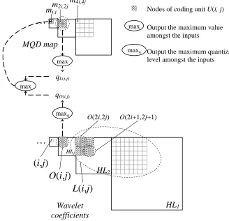
The coding process consists of recursive coding of many small branches of the wavelet trees, and we denote these branches and their related MQD map nodes as BCWT coding units. An example of a BCWT coding unit, U(i,j), is illustrated in Fig. 1, as well as the computation of some of the interim data. For simplicity, only HL-subbands are shown.

-- Step 1: Calculate qO(i,j) , qL(i,j) and mi,j.

-- Step 2: Encode the four offspring coefficients at O(2i,2j).

-- Step 3: Encode the difference qL(i,j) - m2i,2j.

(Repeat Steps 2 and 3 for offspring coefficients at O(2i,2j+1), O(2i+1,2j) and O(2i+1,2j+1).)

-- Step 4: Encode the difference mi,j - qL(i,j).

One can observe that Step 2 is essentially equivalent to processing LIP and LSP in SPIHT, and Step 3 and Step 4 process LIS’s type-A node and type-B node, respectively.

D. One-pass Backward Coding

In the overall encoding process, BCWT simply starts coding the units at level 3; after all of them are coded, BCWT moves one level up; BCWT repeats until the top level is reached; then BCWT encodes the coefficients in the LL-band using simple uniform quantization, the same method used in SPIHT. (Because of the simplicity and common application, we omit the coding of the LL-band in future discussion.)

After all the bits are at the output, we can either re-verse the entire bitstream and transmit, or we can let the decoder read from the end of the stream and go backward. Every step in the decoding is in the exact reverse order of the encoding, therefore the coefficients and MQD map nodes are reconstructed from the highest wavelet level to the lowest.

It is worth mentioning that there are several simple and efficient bit-reversing algorithms available. The entire bit-reversal process can be done “in-place” with no addi-tional memory requirement, and the speed is extremely

fast and usually takes up only 2% of the total core encod-ing time.

E. Coding algorithm

For clarity, we further define the following symbols and operations:

U(i,j): A BCWT coding unit with its root at (i,j).

( )

x

B : The binary code of

 

x

.

( )

n

T

: Shifting function, returns a binary code with a single one at the nth right-most-bit

(

n

≥

0

)

. That is shift-ing binary 1 to the nth bit. e.g.,

T(0) = 00000001; T(5) = 00100000

m n

b

: Clipping function, returns a section of binary

code b, starting from the nth and ending at the mth right-most-bit

(

m

≥

n

≥

0

)

, e.g.,

000 10

000000 42= ;

1101 10

001101 52 =

The steps of encoding a BCWT coding unit U(i, j) are listed in Table I. Note that, when (i,j) is in the level 3 subband, there is an additional step to compute some MQD nodes. Each coding unit above level 3 includes four MQD nodes computed by its children. Level 3 units do not have children. It is also important to note that, once a level 3 unit is coded, these four MQD nodes are no longer needed and are not retained in the MQD map any longer. Therefore, the MQD map of BCWT is only 1/16 the size of the wavelet-transformed-image, not 1/4 the

q

L(i,j)

q

O(i,j)

Wavelet

coefficients

L(i,j)

O(i,j)

(i,j)

MQD map

max

max

maxq

m

i,j

HL

2 HL3

…

…

maxq Output the maximum quantization

level amongst the inputs Output the maximum value amongst the inputs

max

HL

1

Nodes of coding unit U(i, j)

O(2i+1,2j+1) O(2i,2j)

III. BITRATE CONTROL PROBLEM

A. Coarse Bitrate Control in Non-bitplane Codecs

In its original form [9], BCWT provides only coarse bitrate control via the parameter qmin, the minimum quan-tization level. There are large gaps between achievable bitrates, because qmin is an integer dictating the quantiza-tion level to which the binary bits of each coefficient are output.

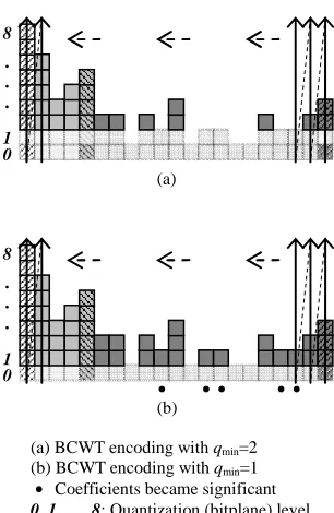
Fig.2 illustrates the cause for the large gaps between achievable bitrates. Both (a) and (b) in the figure repre-sent the BCWT encoding of the wavelet coefficients in a wavelet tree. Note that, for simplicity, only the significant bits of the coefficients are shown in this figure and simi-lar figures in the rest of the paper. Other bits, such as leading bits and sign bits, are omitted.

When qmin is lowered from 2 to 1, not only do we have to output one more bit for each previously significant coefficient, but also there may be many previously insig-nificant coefficients that become siginsig-nificant and thus drastically increase the number of output bits.

Furthermore, the relation between qmin and bitrate is highly image-dependent. It is impossible to precisely pre-dict the bitrate for a given qmin prior to encoding.

A similar bitrate control problem exists in many non-bitplane codecs, such as LTW and Progres.

B. Solution Based on Quantization Step Size Search

Although not explicitly addressed, one solution was hinted at in [8] and was used in LTW’s software package. The basic idea of the solution is to vary the step size for quantizing the wavelet coefficients to achieve different bitrates.

However, the above solution is not suitable for practi-cal applications because it entails an extremely slow process to search for the right step size. The search proc-ess basically is a loop consisting of adjusting step size, quantizing coefficients and encoding. The quantization step size search usually requires more than ten iterations before a reasonably accurate step size can be found.

IV. FINE-GRAINED BITRATE CONTROL

A. Dual Minimum Quantization Level and Quality-index As discussed previously, the large gaps between achievable bitrates for BCWT are mainly due to the fact that qmin must be an integer.

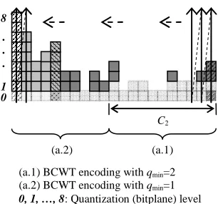
Here we propose an efficient method, i.e., the use of dual minimum quantization levels. Instead of encoding all coefficients with the same qmin, we encode some of the coefficients with qmin=q0+1 and the remaining coeffi-cients with qmin= q0. For example, in Fig. 3, we encode C2 coefficients with qmin=2 and the remainder of the coeffi-cients with qmin=1. It is easy to find the following relation: if C2 increases, fewer encoded bits will be output; if C2 decreases, more encoded bits will be output. Therefore, by changing the value q0 and C2, we can achieve fine-grained bitrates.

TABLE I. ALGORITHM FOR ENCODING ONE BCWTUNIT

1. If (i,j) is in level 3 subband,

{ }

uv l k O v u l

k

q

m

j

i

O

l

k

_,

) , ( ) , (

,

max

:

)

,

(

)

,

(

∈

=

∈

∀

If (i,j) is in level 3 subband, compute the level 2 MQD nodes.

2.

{ }

_kl

j i O l k j i

L

m

q

,

) , ( ) , ( ) ,

(

max

∈

=

Compute the maximum quantization level of the leaves.

3. If

q

L₍i_,j₎

≥

q

_min,

∀

(

k

,

l

)

∈

O

(

i

,

j

)

:

If the leaves are significant, encode the coefficients in the leaves in four groups.

3.1. If

m

_k,l

≥

q

_min,

∀

(

u

,

v

)

∈

O

(

k

,

l

)

: If this group is significant, encode all coefficients in this group.

3.1.1. If

q

_u,v

≥

q

_min, output

sign(

c

_u,v

)

If this coefficient is significant, output its sign.

3.1.2. Output

( )

mkl

q v u

c

B

,

min

,

Encode and output the coefficient.

3.2. Output

( )

(,) min ,, )

max( ,

j i L

l k

q q m l k

m

T

Encode and output the quantization level difference between this group and the leaves.

4.

{

{ }

_{, (, )}

}

) , ( ) , (

,

max

max

kl

,

Lij

j i O l k j

i

q

q

m

∈

=

Compute the maximum quantization level of the descendants.

5. If

m

_i,j

≥

q

_min, output

(

)

ij j i L

m q q j i L

q

T

,

min ) , ( , )

max( ) , (

If the descendants are significant, encode and output the quantization level difference between the leaves and the descendants.

. . .

8

0 1

(a)

(a) BCWT encoding with qmin=2

(b) BCWT encoding with qmin=1 • Coefficients became significant 0, 1, …, 8: Quantization (bitplane) level

. . .

8

0 1

(b)

We define a quality-index, QI,as follows:

C C q

Q_I 2

0+

= , (4)

where C is the total number of wavelet coefficients. Thus, we can use QI as a controlling parameter for the encoding

to achieve fine-grained bitrate control: the smaller the QI,

the higher the bitrates.

Using quality-index as a bitrate controlling parameter has several advantages: (1) no speed penalty; (2) near-linear relation to PSNR; (3) clear physical meaning. The near-linear relation to PSNR is especially useful, because in many applications, quality control is preferable over bitrate control.

However, the relation between quality-index and final bitrates is still image-dependant. For applications that require precise target bitrate control, quality-index is not the best choice. Our second solution to bitrate control will address this problem, but we will first introduce the cod-ing histogram, a new concept upon which our solution is based.

B. Coding Histogram

The coding histogram is simply a mapping that counts the number of encoded bits that fall into different quanti-zation levels (bitplanes). Therefore, if N is the total num-ber of encoded bits, qmax is the maximum quantization level, the coding histogram hq satisfied the following

condition:

∑

=

= max

0

q

q q

h

N . (5)

Fig. 4 shows an example of a coding histogram. In or-der to find the coding histogram, we must know the quan-tization level of each encoded bit. We list the rules for

categorizing the quantization level of encoded bits as follows:

-- Coefficient bits,

( )

mkl q v u

c

B ,

min

, , are of quantization

lev-els from mk,j to qmin.

-- Sign bits,

sign(

c

_u,v

)

, are of quantization level qu,v.

-- Difference bits,

( )

(,) min ,, )

max( ,

j i L

l k q

q m l k

m

T , are of

quantiza-tion levels from qL(i,j) to max(mk,l, qmin). -- Difference bits,

(

)

ij

j i L m

q q j i L

q

T ,

min ) , ( , )

max( ) ,

( , are of

quantiza-tion levels from mi,j to max(qL(i,j), qmin).

C. Bitrate Control based on Coding Histogram

The goal of our second bitrate control solution is to provide the ability to encode to a specified target bitrate. In other words, given a target bitrate, we need to find out: (a) q0 for qmin and (b) when to use q0 for encoding and when to use q0+1.

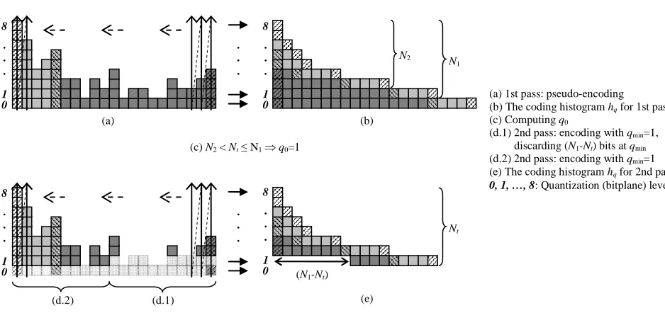
To achieve this goal, we use a two-pass coding based on the coding histogram. In the first pass, BCWT per-forms a “pseudo-encoding” with qmin set to 0. Pseudo-encoding means we do not output any of the bits but only generate the coding histogram. Then q0 is the value that satisfies the following inequality:

0 01 t q

q N N

N ₊ < ≤ , (6)

where Nt is the target number of bits, and

∑

+ = + =

max 0 0

1 1

q

q q

q

q h

N , (7)

∑

=

= max

0 0

q

q q

q

q h

N . (8)

In the second pass, we perform a true encoding using qmin=q0, but the first ( )

0 t

q N

N − bits at quantization level qmin will not be output. Discarding those bits is equivalent to encoding the related coefficients using q0+1. Note that

BCWT encodes the coefficients backward; therefore we discard the first (Nq₀ −Nt)bits in the bitstream, not the last bits. Fig.5 is an example of the two-pass encoding based on coding histogram.

The speed penalty of the above bitrate control solution is the “pseudo-encoding” in the first pass, which costs roughly the same time as a true encoding. Compared with the penalty based on a quantization step size search, the “pseudo-encoding” has a fixed coding penalty, whereas the quantization step size search has an image-dependent penalty that is usually more than ten times higher than the former.

. . .

8

0 1

(a.2) (a.1)

(a.1) BCWT encoding with qmin=2

(a.2) BCWT encoding with qmin=1

0, 1, …, 8: Quantization (bitplane) level

C2

Figure 3. Dual minimum quantization level

. . .

. . .

8

0 1

. . .

8

0 1

(a) (b) (c)

(a) BCWT encoding (b) Counting the encoded bits (c) The coding histogram hq

0, 1, …, 8: Quantization (bitplane) level

V. EXPERIMENTAL RESULTS

Experiments were conducted using a PC with a 2.21GHz AMD Athlon64 3200+ Processor and Window XP. Currently, only Java implementation is available for the BCWT with fine-grained bitrate control, whereas co-decs such as SPIHT, LTW and Progres do not offer Java implementation. Therefore, we compared BCWT only with JPEG2000 in this paper.

The codecs tested in the experiments are Java imple-mentations: BCWT, version 1.01, binary uncoded; JPEG2000 (JJ2000), version 4.1, with arithmetic encod-ing. Results for the standard test image, “monarch” (768x512, 24-bit RGB), are listed in the Tables II and III. Note that, because JJ2000 does not report core coding time, all times shown in the tables are end-to-end, which means file I/O and DWT are included.

Table II shows the time to encode the tested image to various bitrates, along with the corresponding quality-index of each bitrate. For BCWT, the encoding times for using two different controlling parameters are shown. Using quality-index as the controlling parameter has no speed penalty and thus it yields the fastest coding speed, which is about 2X faster than JPEG2000. Using target bitrate as the controlling parameter has a small speed penalty (ranging form 40% to 56%), but it is still faster than JPEG2000 (about 18%).

Table III shows the time and PSNR to decode at vari-ous bitrates. BCWT is about 4X faster than JPEG2000, and the PSNR performances are very close between the two codecs. BCWT results in slightly worse PSNR at 1.00 bpp and below, but slightly better PSNR at 1.50 bpp and above. It is important to point out that although BCWT is binary uncoded, it outperforms arithmetic-coded JPEG2000 in 4 out of 6 dearithmetic-coded bitrates.

TABLE II. ENCODING TIME

Encoding Time (ms)

BCWT

Bitrate (bpp)

Quality-index

Bitrate QI

JPEG2000

0.50 4.898831 343 219 422

1.00 3.616604 343 234 422

1.50 2.796753 344 235 422

2.00 1.948839 359 250 437

2.50 1.747084 375 265 453

3.00 1.572971 391 281 468

TABLE III. DECODING TIME AND PSNR

Decoding Time (ms) PSNR (dB) Bitrate

(bpp) _{BCWT JPEG2000 BCWT JPEG2000}

0.50 171 390 33.15 33.81

1.00 187 547 38.03 38.84

1.50 195 656 41.31 40.80

2.00 203 813 42.97 42.82

2.50 212 984 44.05 43.81

3.00 219 1094 45.49 44.72

VI. CONCLUSION AND FUTURE WORK

In this paper, we have presented two solutions to the coarse bitrate control problem in the original BCWT, together with three new concepts, namely dual minimum quantization levels, quality-index and coding histogram.

One of the solutions is based on dual minimum quan-tization levels and allows fine-grained bitrate control via quality-index. The other solution is based on coding his-tograms and allows BCWT to encode to any target bitrate. Different applications may choose from these two solu-tions based on their requirements. Controlling via quality-index is best suited for applications where quality control is preferable over bitrate control or where fast coding speed is preferred. Controlling via target bitrate entails a small speed penalty but is best suited for applications where precise bitrate control is necessary.

. . .

. . .

8

0 1

. . .

8

0 1

(a) (b)

(a) 1st pass: pseudo-encoding

(b) The coding histogram hq for 1st pass

(c) Computing q0

(d.1) 2nd pass: encoding with qmin=1,

discarding (N1-Nt) bits at qmin

(d.2) 2nd pass: encoding with qmin=1

(e) The coding histogram hq for 2nd pass

0, 1, …, 8: Quantization (bitplane) level

. . .

. . .

8

0 1

. . .

8

0 1

N2 _N

1

Nt

(N1-Nt)

(d.2) (d.1) (e)

(c) N2 < Nt≤ N1⇒ q0=1

In parallel to this work, we have successfully modified BCWT so that it could generate a rate-embedded bit-stream [10]. We will combine these modifications so that BCWT can provide all these features: resolution-scalability, rate-scalability and fine-grained bitrate con-trollability.

ACKNOWLEDGMENT

This research has been partially supported by a con-tract from the National Library of Medicine (concon-tract #467-MZ-301975) and a grant from Texas Advanced Technology Program (grant #003644-0034-2003).

REFERENCES

[1] J.M. Shaprio, “Embedded Image Coding Using Zerotrees of Wavelet Coefficients,” IEEE Trans. on Signal Process-ing, vol. 41, pp. 3445-3459, Dec. 1993.

[2] A. Said and W.A. Pearlman, “A New Fast and Efficient Image Codec Based on Set Partitioning in Hierarchical Trees,” IEEE Trans. on Circuits and Systems for Video Technology, vol. 6, pp. 243-250, 1996.

[3] H. Danyali and A. Mertins, "Highly Scalable Image Com-pression Based on SPIHT for Network Applications," Proc. of IEEE Int. Conf. on Image Processing, Rochester, NY, pp. 217-220, Sept. 2002.

[4] M.G. Ramos and S.S. Hemami, "Activity Selective SPIHT Coding," Proc. of SPIE Visual Comm. and Image, San Jose, CA, Jan. 1999.

[5] F.W. Wheeler and W.A. Pearlman. “SPIHT image com-pression without lists”, Proc. of IEEE ICASSP 2000. [6] W.A. Pearlman, "Trends of Tree-Based, Set Partitioning

Compression Techniques in Still and Moving Image Sys-tems (Invited, keynote paper)," Proc. of Picture Coding Symposium, Seoul, Korea, pp. 1-8, April 2001.

[7] J. Oliver and M.P. Malumbres, "Fast and Efficient Spatial Scalable Image Compression using Wavelet Lower Trees," Proc. of IEEE Data Compression Conf., pp. 133-142, Mar. 2003.

[8] Y. Cho, W. A. Pearlman, and A. Said, Low Complexity Resolution Progressive Image Coding Algorithm: Progres (Progressive Resolution Decompression), IEEE Int. Con-ference on Image Processing 2005 (ICIP 2005), Vol: III, pp. 49-52, 2005.

[9] J. Guo, S. Mitra, B. Nutter, and T. Karp, “A Fast and Low Complexity Image Codec based on Backward Coding of Wavelet Trees”, IEEE Proceedings of Data Compression Conference 2006 (DCC2006), pp. 292-301, Mar. 2006. [10]J. Guo, S. Mitra, T. Karp, and B. Nutter, “A Resolution

and Rate Scalable Image Subband Coding Scheme with Backward Coding of Wavelet Trees”. To be presented at IEEE Asia Pacific Conference on Circuits and Systesms, Singapore, December 2006.

Jiangling Guo received his B.S. and M.S. degree in

Elec-tronics Engineering from Jinan University, Guangzhou, P.R. China in 1994 and 1998. He received his Ph.D. degree in Elec-trical Engineering from Texas Tech University, Lubbock, USA in 2005. He is currently a faculty member at the School of In-formation Science and Technology, Beijing Institute of Tech-nology at Zhuhai (ZHBIT), Zhuhai, P.R. China. Before he joined ZHBIT, he was Senior Research Associate at the

De-partment of Electrical and Computer Engineering at Texas Tech University, USA. His research interests are image compression and video compression, image processing, pattern recognition and computer graphics.

Sunanda Mitra is a Horn Professor in the Department of

Elec-trical and Computer Engineering at Texas Tech University (TTU) and has been the Director of the Computer Vision and Image Analysis Laboratory in the Department of Electrical and Computer Engineering since 1988. Dr. Mitra received her B.S. and M.S. degrees in physics from Calcutta University, India in 1955 and 1957, and her D. Sc. (Doctors der Naturwissenshaften) in Physics from Phillips University in Marburg, Federal Repub-lic of Germany in 1966. Prior to taking the faculty position at TTU in 1984, Dr. Sunanda Mitra has worked as a research sci-entist at TTU, TTU Health Sciences Center, and as a visiting faculty member at the Mount Sinai School of Medicine in New York. Prof. Mitra served on the Board of Scientific Counselors (BoSC) of the National Library of Medicine from 1997-2001. She has also chaired the Technical Committee of Computational Medicine of the IEEE (Institute of Electrical and Electronics Engineers) Computer Society and the Steering committees (1998-2001) for IEEE Symposia on Computer Based Medical System (CBMS). She is also on the program committee of the International Medical Imaging Symposium on “Image Process-ing” sponsored by the SPIE (The International Society for Opti-cal Engineering). Dr. Mitra's specialization includes mediOpti-cal image segmentation and analysis, data compression, 3-D model-ing from stereo vision, pattern recognition, neural networks, and neuro-fuzzy control and recognition.

Brian Nutter received his Ph.D. degree in Electrical

Engineer-ing from Texas Tech University in 1990 and his B.S.E.E. also from TTU in 1987. Dr. Nutter has worked in a variety of senior engineering and technical management roles at rapid prototyp-ing firms 3-D Systems (Valencia, CA) and Soligen (Northridge, CA). He developed and implemented a number of geometric software algorithms, user interfaces, and hardware control ap-plications for stereolithography and Direct Shell Production Casting. He was the Vice President of Engineering at Willow-Brook Technologies (Van Nuys, CA), which developed distrib-uted peer to peer Voice-Over-IP telephone equipment. He has been an Associate Professor in ECE at TTU since 2002, re-searching in distributed control systems, embedded systems, superresolution and autostereoscopy. Dr. Nutter is an IEEE member and a registered Professional Engineer.

Tanja Karp received the Dipl.-Ing. degree in electrical