Scenario Analysis for Image Classification using Multi-objective
Optimization
ELIANAPANTALEÃO1
LUCIANOVIEIRADUTRA1
SANDRASANDRI2
INPE - Instituto Nacional de Pesquisas Espaciais CAP - Curso de Pós-Graduação em Computação Aplicada Av. dos Astronautas, 1758 12227-010 - São José dos Campos(SP)- Brazil
1
(elianap,dutra)@dpi.inpe.br 2
Abstract. In a typical image classification task, the analyst decides beforehand the number of classes and which image channels to use. If there is a need to modify the classes or data channels, it is necessary to start over. This paper proposes a scenario analysis tool for the task of image classification as a way of automating this process. Each scenario represents the parameters that will be used in a complete super-vised classification task, including training and classification. The proposed method uses multi-objective optimization to evaluate different sets of attributes and classes, and presents the compromising solutions, regarding the user objectives. A class hierarchy structure is used to generate different class sets, and the system attempts to find the most appropriate combinations of class and attribute sets. In this work, the system is applied to remote sensing problems and we consider three objectives: the best classification accuracy, the smallest attribute set and the biggest class set. The system shows the compromising combi-nations of class and attribute sets, along with the accuracy on a testing sample. The user can then choose which combination to use for the image classification.
Keywords:image classification, multi-objective optimization, class hierarchy, remote sensing.
(Received September 24th, 2012 / Accepted January 24th, 2013)
1 Introduction
This paper proposes a scenario analyst intended to be used for remote sensing applications. Remote sensing is the process of collecting data about objects or land-scape features without coming into direct physical con-tact with them. Remotely sensed data are usually stored as arrays of two-dimensional data referred to as im-ages. Pattern recognition aims to associate categories or classes to objects represented by a set of measure-ments, named feature vector or pattern. In the task of image classification for remote sensing applications, the features usually correspond to the image itself, that is, the digital values of the image matrices. Derived infor-mation such as texture, band math and principal
com-ponent analysis can also be used [10], [13], [1].
a direct influence on the accuracy of pattern recognition applications [19].
The pattern recognition task of assigning classes to feature vectors can be supervised, semi-supervised or unsupervised. In supervised learning, the user gives the classifier a training set of labeled examples for each class, which are used to estimate the class model or boundaries between classes. After that, it is possible to assign each unknown pixel or region to the appropri-ate class. All classifications performed in this work use supervised learning.
Several attempts have been made to improve classi-fication by automatically choosing the input elements. In [2], decision trees are used to find a compromising solution for class set specificity and classification accu-racy. In [11], the authors use a genetic algorithm to se-lect the features and, concurrently, find the best param-eters for a support vector machine classifier. A multi-objective optimization technique is used by [17] to se-lect features in data bases. The addition of new vari-ables and objectives in these methods can not be done with little effort. In [2], only the classes are consid-ered, and [17] varies only the feature subset. In [11], the classes are not considered. Besides, the objectives are combined in an equation with weights that reflect how important the user considers each one of the objectives, and these weights have to be set before the optimization process.
In the method proposed in this paper, we consider as part of the varying scenario a set of features and a set of classes, as in Figure 1. The idea is to generate different feature and class sets and evaluate the performance of these different scenarios in the image classification task.
Figure 1: Scenario elements
In order to decide what a good classification is, sev-eral types of objectives can be considered. The system is flexible to allow the addition of new objectives with little programming effort. In this implementation we considered three: the best classification accuracy, the smallest attribute set and the biggest class set, meaning more specific classes. Other examples could be the best generalization power, reduced classification time or in-creased uniformity inside some predefined size window.
2 Multi-objective optimization
A multi-objective optimization approach is necessary when there are at least two conflicting objectives aimed for a problem and there is no unique solution that is best for all objectives [9]. In this case, one possible tactic is to find the set of all non-dominant solutions, referred to as the Pareto set approach [20].
In the multi-objective optimization problem shown in the formulation (1), the goal is to find the best vector
~xof N variables, to minimizeM objective functions. The feasible searching space is limited by lower and upper bounds for each variablexi, and alsoJinequality
andKequality constraints [6].
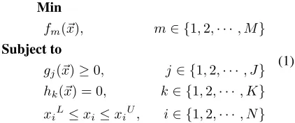
Min
fm(~x), m∈ {1,2,· · ·, M} Subject to
gj(~x)≥0, j ∈ {1,2,· · · , J}
hk(~x) = 0, k∈ {1,2,· · · , K}
xiL≤xi ≤xiU, i∈ {1,2,· · · , N}
(1)
Using the Pareto set approach, the aim is to findS
non-dominant solutions~xs,S ≥ 1. Dominance is
de-fined as the relationand a solutionx~s1is said to
dom-inate another solutionx~s2if both conditions (2) and (3)
are true.
(∀m)(fm(x~s1)≤fm(x~s2)) (2)
(∃m)(fm(x~s1)< fm(x~s2)) (3)
Condition (2) states that there is no objective func-tion wherex~s1is worse thanx~s2and condition (3) states
thatx~s1is strictly better thanx~s2in at least one
objec-tive [3]. If there is at least one pair(m1, m2)for which
fm1(x~s1)< fm1(x~s2)andfm2(x~s1)> fm2(x~s2)then
neither of the solutions dominates the other, because it is not possible to say that one solution is better than the other for both objectives. Since it is a minimization problem,x~s1is a better solution for objective function
fm1, whilex~s2 is better for fm2. The Pareto set is a
set of viable solutions where none of them dominates any of the others [6] and is formally defined in expres-sion (4).
P∗={x~1| 6 ∃x~2:x~2x~1)} (4)
In the Pareto set, the elements are solutions, or val-ues for the minimization problem variables. The set of the objective functions values for the Pareto set is called Pareto frontier and is given by expression (5).
The image classification task can be seen as a multi-objective problem, because choosing more spe-cific classes usually results in lower accuracy, so it makes sense to find compromising solutions. Particu-larly in remote sensing applications, one typical use of classification is to derive a land cover or land use map [16]. How specific this map can be, given the available data, is a question frequently faced by human analysts. Choosing to discriminate only “agriculture” instead of “corn” and “sugarcane” usually requires less attributes, and leads to a more accurate map, with less confusion between classes. Descending in class hierarchy makes accuracy worse, but depending on how worse that is, it can be considered a better map, because it is more spe-cific; and all this is affected by the number of features used.
When we try to minimize the number of features while maximizing the classification accuracy and de-scend as low as possible in the class taxonomy, we are doing multi-objective optimization. They are conflict-ing objectives because optimizconflict-ing one of them degrades at least one of the others [19], [16]. There is no unique optimal solution, but a set of solutions representing a trade-off surface among several objectives. None of these solutions can be considered better than the others with respect to all goals simultaneously. It is the user, with some higher level information, who can choose the one to be adopted [6]. In the end of the process of this proposed method, a report with the evaluation of the scenarios which produced the trade-off results is gen-erated. Therefore, the final report contains the descrip-tion and the classificadescrip-tion result analysis of the scenar-ios which have the best compromise of the three goals.
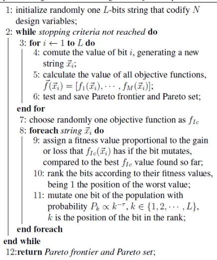
In this work, the implementation of the multi-objective optimization solution was based on the M_GEO algorithm [7], a multi-objective version of the Generalized Extremal Optimization (GEO) algo-rithm [8]. GEO is an evolutionary algoalgo-rithm where the species are represented by a string of bits that encodes the variables of the optimization problem. Each bit is forced to “evolve” with a probability that is proportional to its fitness. The M_GEO algorithm is shown in Fig-ure 2.
The only free parameter to adjust, theτin Figure 2, step 11, controls the determinism level of the search, from completely random (τ = 0) to a deterministic search (τ → ∞). For each specific problem, there is a value forτthat maximizes the search efficiency [7].
The species were implemented as a bit string rep-resenting two variables, the feature and the class set, according to the scenario definition presented in Sec-tion 3.
Figure 2: M_GEO algorithm
3 Scenario Definition
In the context of this work, a scenario consists of a fea-ture and a class set, as in Figure 1. These variables val-ues are altered by the scenario generator. A classified image is generated when a classifier uses the scenario components to classify an image (Figure 3). The idea in this system is to evaluate different scenarios and find the compromising ones according to two or more ob-jectives sought for the classification result.
Figure 3: Classification task using scenario
Formally, we define scenario as a pairS = (Φ,Ω), whereΦis the attribute or feature set andΩis the class set. WhenSis applied to imageI, the classified image
IS is generated.
the user expects the classifier to find in the image. The ideal is that the hierarchy is based on semantic informa-tion, not on attributes values or classes spectral behav-ior. However, if this information is not available, it is possible to generate the hierarchy automatically, using information from the available features [14].
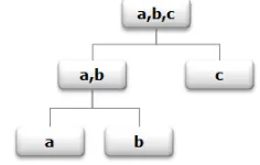
Figure 4: Example of a class tree
The labeled samples provide information about available features, allowing the scenario generator to build different attribute combinations, the different sets Φ. Any subset of the initial set of all attributes can be generated, except the empty set, since it is not possible to perform a classification with no features.
The generation of class setsΩis guided by a class tree. LetΓ be the set of all the most specific classes, those that would be the class tree leaves. If no class tree was used, any partition of Γ could be used as a set Ω except the one where all classes are included in the same subset (the root of the class tree). If we used this partition, no classification would take place, since there would be only one class including all sam-ples. But in this work, we use the class tree to exclude other semantically less meaningful partitions. For ex-ample, consider the class tree in Figure 4, built from Γ = {a, b, c}. There are five possible partitions for Γ:{{a, b, c}},{{a, b},{c}},{{a, c},{b}},{{a},{b, c}} and {{a},{b},{c}}. The first one is the set of all classes, therefore cannot be used as Ω. And only {{a, b},{c}} and {{a},{b},{c}} are allowed by the class tree in Figure 4. It is not possible to merge classes
bandcin the same class, leavingaalone, because this is not how the tree is structured.
4 Scenario Analyst
The scenario analyst uses a multi-objective optimiza-tion algorithm to find compromising scenarios, accord-ing to the intended objectives. Figure 5 shows the methodology steps implemented by the system.
The implementation of the scenario generation fol-lowed the model stated in Section 3. The string that is used to represent these design variables is aL-bit string, whereL=F+C,Fis the number of available features
Figure 5: System architecture
andCis the total number of all classes considered, in-cluding all leaves and internal nodes of the class tree, except the root.
The only attribute set constraint is to be non-empty, so, if the scenario generator is altering the value of the firstFstring bits and an all-zeroF-bits substring is gen-erated, it is ignored, and another one is produced. Any other combination is allowed.
As for the lastCbits, the constraints are more com-plex, because they consider the class hierarchy that guides the class set generation. There are two con-straints that must be true for all classes in the hierarchy:
• If a class is included in a class set, then none of its ascendants or descendants can be in the set at the same time.
• If a class is not included in a class set, then either one of its ascendants or descendants must be in the set.
With these two constraints, the class set is guaran-teed to follow the proposed formal model. In practice, it guarantees that no class is ever removed from the sce-nario; it either joined its siblings forming a superclass or was divided into subclasses.
we initialize the system with the complete scenario, the one where all features are used, and the most specific classes are discriminated.
5 Case Study
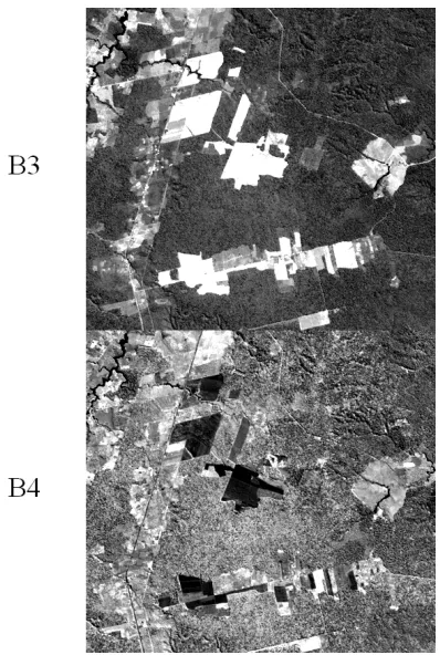
As a system application, the land cover was extracted from a Landsat-5 image []. The study area is located in the Amazon region of Brazil, in Para state. The op-tical image is from sensor TM (Thematic Mapper) and was acquired on June, 29th, 2010. We use 6 bands: B1-B5 and B7. The image has 30 meters of spatial res-olution, 8 bits of radiometric resolution and 1672000 pixels, structured in 1900 lines and 880 columns.
The original image can be obtained from INPE Im-age Catalog [12]. The field samples were assigned to a previously segmented image, and only a spatial subset was used, in order to fit other data source. The com-plete processing of the input data is described in [15]. The channels B3 and B4 from the whole used image can be seen in Figure 6 and a more detailed view can be observed in the subset shown in Figure 7.
Figure 6: Bands 3 and 4 from TM image
The classes to be discriminated originated from sev-eral field works performed in 2010 and include some types of forests, agriculture and pasture. A class tree was built by a remote sensing specialist and can be seen in Figure 8. Table 1 shows the meaning of the classes and the size of the available samples in pixels.
Three objective functions were considered: the ac-curacy of the classification and both sizes of the class
Figure 7: Detail of bands 3 and 4 from TM image
Table 1: Meaning of the classes from the class tree
class meaning sample size
OR old regeneration 2518
DF degraded forest 2306
IntR intermediate regeneration 453
PF primary forest 7035
EF exploitation forest 3635
NR new regeneration 794
DP dirty pasture 828
FL7 fallow land 7-24 months 269
FL fallow land 1306
S40 soybean 40 days 134
S100 soybean 100 days 581
CPI clean pasture and inaja 753
CP clean pasture 906
and the feature set. The Maximum Likelihood (ML) classifier was used to perform the pixel wise, supervised classifications.
Several ways to measure accuracy are available, but there is no agreement about which one is the best. Most quantitative methods use the confusion matrix [18] de-rived from classification data and reference data. The kappa coefficient, presented by Cohen [4], is a widely used measure in remote sensing applications.
In this application, we use kappa coefficient (κ) to assess the agreement between the result of the classifi-cation and the reference data (the labeled samples). Our three objective functions are shown in the set of equa-tions (6).
f1 =−|Ω|
f2 =|Φ|
f3 =−κ
(6)
The negative signs inf1andf3are needed because
we solve it as a minimization problem, and we want to maximize these values. We have only one restriction: the value ofκmust be at least0.5so the classification can be considered satisfactory.
The resulting Pareto set and frontier can be observed in Table 2. The elements of theΩisets,ifrom 1 to 6,
are in Table 3. The size of theΩsets was included in Table 2 for emphasis. The notationP F.EF means that the samples from the two classesP F andEFwere all relabeled to one single class, forming their parent class shown in the class tree.
Six different class sets were included by the system in the Pareto set, and five different feature sets. The best feature set, that is, the smallest one, is1,2,5,6, which suggests these bands are the most powerful to discrimi-nate the user classes inΩ3. The scenario with all classes
and all features has a low kappa,0.5295, and removing one feature (thus improvingf2) does not make it better.
A much better kappa is obtained when the user is satis-fied with discriminating only the top four classes from the class tree (Ω6).
Table 2: Selected scenarios
bands classes |Φ| |Ω| κ 1,2,3,4,5,6 Ω1 6 13 0.5295
1,3,4,5,6 Ω1 5 13 0.5181
1,2,3,5,6 Ω1 5 13 0.5181
1,2,3,4,6 Ω1 5 13 0.5181
1,2,3,4,5,6 Ω2 6 12 0.5694
1,2,5,6 Ω3 4 12 0.5249
1,2,3,4,5,6 Ω6 6 4 0.7986
1,2,4,5 Ω6 4 4 0.7957
1,2,3,4,5,6 Ω4 6 10 0.5865
1,2,4,5,6 Ω5 5 7 0.6401
Table 3:Ωelements
set elements
Ω1 AP,AP7,RA,FP,PL,RI,S40,S100,FD,FPE,PLI,RInt,PS
Ω2 AP,AP7,RA,PL,RI,S40,S100,FD,FP.FPE,PLI,RInt,PS
Ω3 AP,AP7,RA.FD,PL,RI,S40,S100,FP,FPE,PLI,RInt,PS
Ω4 RA.FD,RInt,FP.FPE,RI,PS,AP7,S40.S100,AP,PL,PLI
Ω5 RA.FD,RInt,FP.FPE,RI.PS.AP7,S40.S100,AP,PL.PLI
Ω6 RA.RInt.FD.FP.FPE,RI.PS.AP7,S40.S100.AP,PL.PLI
The image was classified using the scenarios of Ta-ble 2. Figure 9 shows the detailed view of three classi-fied images. In order to obtain the classification in Fig-ure 9a, all 13 classes were used, and all 6 image bands. The accuracy for this classification isκ = 0.5295and the classified image has a lot of isolated pixels, sug-gesting great confusion between classes. Figure 9b was generated with the class setΩ5, with 7 classes, and 5
bands (1,2,4,5,6) were used. Even with fewer bands, the accuracy of this classification was better (κ= 0.6401), which can be explained by the use of fewer classes. Fig-ure 9c used class setΩ6(4 classes) and only 4 bands,
obtainingκ= 0.7957. This last classified image shows a better definition of the discriminated classes, with less isolated pixels.
The graph in Figure 10 shows the variation of the three objectives for the eight different solutions in the Pareto set. The optimal solutions of each function are marked. The values ofkappawere multiplied by 10 so the variation could be placed in the same range as the other objective functions.
Figure 9: Detail of classified images for scenarios with (a) 13 classes, 6 bands; (b) 7 classes, 5 bands; and (c) 4 classes, 4 bands
Figure 10: Variation of the objective functions
give a good kappa.
6 Comments and Future Work
The image classification task can be improved by a choice of the best classification scenario. An automated analyst makes it easier to consider the possible options for generating different scenarios. The multi-objective optimization proved to be a good method to solve this issue. Finding the best Pareto set of compromising sce-narios will help the user to consider the best possibili-ties. The final choice of the best result will depend on the user application, resources availability and model restrictions. Although this method was created to be used in remote sensing applications, it may also be ap-plied to other pattern recognition problems.
The flexibility aimed for the system was reached with respect to the definition of new objectives to be op-timized and the selection of the project variables among the ones already coded. The addition of new variables, however, requires more computational effort. New data structures and means to generate their values authomat-ically need to be developed.
As future steps, we will add more variables to the scenario, such as the type of classifier and its parame-ters, and include other objective functions, like the gen-eralization power. We also consider using a priority value to the classes, thus reducing the possibility of the system eliminate the ones that are more important to the user.
Acknowledgements
References
[1] Bishop, C. M. Pattern recognition and ma-chine learning. Information Science and Statis-tics. Springer, New York, NY, 2006.
[2] Chen, Y.-L., Hu, H.-W., and Tang, K. Construct-ing a decision tree from data with hierarchical class labels. Expert Systems with Applications, (36):4838–4847, 2009.
[3] Coello, C. A comprehensive survey of evolutionary-based multiobjective optimization techniques.Knowledge and Information Systems: An International Journal, 1(3):269–308, 1999.
[4] Cohen, J. A coefficient of agreement of nominal scales. Educational and Psychological Measure-ment, (20):37–46, 1960.
[5] Dash, M. and Liu, H. Feature selection for classi-fication. Intelligent Data Analysis, 1(3):131–156, 1997. Cited By (since 1996): 255.
[6] Deb, K.Multi-objective optimization using evolu-tionary algorithms. John Wiley and Sons, Chich-ester, 1 edition, 2001.
[7] Galski, R. L. Desenvolvimento de versões ap-rimoradas híbridas, paralela e multiobjetivo do método da otimização extrema generalizada e sua aplicação no projeto de sistemas espaciais. PhD thesis, Instituto Nacional de Pesquisas Espaciais, São José dos Campos, 2006-09-22 2006.
[8] Galski, R. L., Souza, F. L. d., Ramos, F. M., and Muraoka, I. Application of a new hybrid evo-lutionary strategy to spacecraft thermal design. In Anales...Genetic and Evolutionary Computa-tional Conference (GECCO), 2004.
[9] Goicoechea, A., Hansen, D., and Duckstein, L. Multiobjective decision analysis with engineering and business applications. John Wiley and Sons, New York, 1 edition, 1982.
[10] Gonzalez, R. C. and Woods, R. E. Digital image processing. Prentice Hall, Upper Saddle River, NJ, 2 edition, 2001.
[11] Huang, C.-L. and Wang, C.-J. A GA-based feature selection and parameters optimization for support vector machines. Expert Systems with Applica-tions, 31(2):231–240, 2006.
[12] INPE. Image Catalog. National Insti-tute for Space Research, 2004. Brazil, http://www.dgi.inpe.br/CDSR/.
[13] Jensen, J. R. Remote sensing of the environment: an Earth resource perspective. Prentice Hall, Up-per Saddle River, NJ, 2 edition, 2007.
[14] Negri, R. G. Avaliação de dados polarimétricos do sensor alos palsar para classificação da cober-tura da terra da amazônia. Master’s thesis, In-stituto Nacional de Pesquisas Espaciais, São José dos Campos, 2009-05-19 2009.
[15] Pereira, L. d. O. Avaliação de métodos de inte-gração de imagens ópticas e de radar para a clas-sificação do uso e cobertura da terra na região amazônica. Master’s thesis, Instituto Nacional de Pesquisas Espaciais (INPE), São José dos Cam-pos, 2012-08-27 2012.
[16] Schowengerdt, R. A.Remote sensing: models and methods for image processing. Academic Press, San Diego, 3 edition, 2007.
[17] Spolaôr, N. Aplicação de algoritmos genéticos multiobjetivo ao problema de seleção de atribu-tos. Dissertação (mestrado em engenharia de in-formação), UFABC, Santo André, 2010.
[18] Story, M. and Congalton, R. G. Accuracy as-sessment: A user’s perspective. Photogrammet-ric Engineering and Remote Sensing, 52:397–399, 1986.
[19] Theodoridis, S. and Koutroumbas, K. Pattern recognition. Academic Press, San Diego, 3 edi-tion, 2006.