The welfare effects of lotto: evidence from the UK
*Lisa Farrell, Ian Walker
Department of Economics, Keele University, Staffs ST5 5BG, UK Received 30 April 1997; received in revised form 28 July 1998
Abstract
This paper estimates the demand for lottery tickets using pooled cross section data that contain individual incomes and extensive information about characteristics. One of the cross sections corresponded to a draw which was a ‘double rollover’ – the jackpot was enhanced by adding the two previous draws’ jackpots which had not been won. Together, these datasets provide sufficient observations facing different ‘prices’ to allow us to estimate the ‘price’ elasticity as well as the income elasticity of demand. We estimate Tobit and other specifications and use the estimates to evaluate the welfare effects arising from the introduction of the lottery. 1999 Elsevier Science S.A. All rights reserved.
Keywords: Gambling; Lottery; Lotto
JEL classification: D12; H30; D80; C21
1. Introduction
Lotteries typically offer large prizes at long odds. Most countries now have lotteries and, invariably, they raise considerable amounts of revenue. These are often state owned monopolies where the revenue in excess of costs is used as tax revenue (sometimes hypothecated) and in other cases these are regulated with tax and other deductions being contractually specified proportions of revenue. The design and taxation of lotteries have attracted some attention, and the ‘price’ and income elasticities are important considerations for design: the income elasticity
*Corresponding author. Tel.: 144-1782-583111; fax: 144-1782-717577; e-mail: [email protected]
0047-2727 / 99 / $ – see front matter 1999 Elsevier Science S.A. All rights reserved. P I I : S 0 0 4 7 - 2 7 2 7 ( 9 8 ) 0 0 0 8 9 - 9
determines how regressive (or otherwise) lotteries might be in raising revenue for the government (or other body), while the price elasticity is important for efficiency considerations.
The ‘price’ elasticity of demand for lottery tickets shows how demand varies with the expected value, V, of the return from a ticket and it is this elasticity that is relevant to the design of the lottery and one factor in determining how it should be taxed. That is, it tells us how demand would vary in response to changes in the
design of the lottery – in particular, the tax rate on the lottery or the nature of the
prizes. Previous work has attempted to estimate this elasticity by looking at how aggregate sales vary across different lottery designs: for example, across time in response to changes in the design of a lottery, or across regions which have
1
different lottery designs. However, time series changes have been few and far between, and may themselves be endogenous responses to disappointing (or booming) sales. Regional variations in design may be associated with unobserv-able cross region differences in factors affecting lottery play as well as varying systematically with population size. Farrell et al. (1996), (1997) estimate the
2
elasticity of sales with respect to rollover induced variation in the expected value of holding a ticket using time series data on sales. However, time series analysis is not able to identify the income elasticity because there is such little variation in income over the short run of data that is typically available.
There have been relatively few studies of lottery demand based on microdata (see Scott and Garen, 1994, and references therein) and none are able to estimate
3
the price elasticity of demand because of the absence of ‘price’ variation. Here, the identification of the elasticity of sales with respect to the ‘price’ of a ticket again relies only on variations in the expected value which arise exogenously because of rollovers. That is, we exploit the changes in the return to a ticket induced by ‘rollovers’ which occur when the major prize (the ‘jackpot’) in one week is not won and gets added to the prize pool for the subsequent week. This makes the expected return to a lottery ticket in the rollover week higher in a very specific way. It is only by comparing rollover with non-rollover weeks that we can reveal the appropriate demand elasticity – rollovers shift the (inverse) supply function that induces a movement along the demand curve.
The fact that we rely on rollovers for identification causes us a difficulty: rollovers should occur with relative infrequency so we may have insufficient data to obtain a reliable estimate. However, one of the startling features of the UK lottery (and others) is that it exhibits many more rollovers than could have been
1
See Cook and Clotfelter (1993) (Table 2), for example. Several studies report price elasticities in a narrow band around 1.2: see, for example, DeBoer (1985) and Vrooman (1976).
2
A rollover occurs when a prize (typically the jackpot) is not won in a given draw and it is then added to the prize pool for the next draw.
3
Scott and Garen (1994) use data for an ‘Instant’ lottery where individuals purchase a ‘scatchcard’ which immediately reveals whether a prize has been won. Such games do not feature rollovers.
generated by statistical chance: instead of there being approximately one rollover
4
every two years there have been almost 20 times as many. Thus, the availability of several surveys, each covering a different draw, gives rise to the possibility of being able to compare the behaviour of individuals who play in rollover draws
5
with that of those who play in regular draws to deduce a ‘price’ elasticity. Earlier work used rollover-induced changes in V on sales to infer a ‘price’ elasticity of demand with time series data (see, for example, Gulley and Scott, 1993; Farrell et al., 1997).
There are two novel features of the paper. Most importantly, this is the only paper to estimate price and income elasticities using microdata. Indeed, this is the first paper to explicitly construct a ‘price’ variable from microdata that allows for the effect of rollovers. Moreover, the estimates are obtained using estimation methods that acknowledge the limited dependent nature of the problem: that is, that many individuals choose not to participate. Secondly, we use the estimates that we obtain to impute the welfare effects arising from the introduction of the lottery into the UK.
The plan of the paper is as follows. In Section 2 we outline the relevant theory relating to the factors determining the expected value of holding a lottery ticket. We contrast how the expected return varies with sales when there is a rollover and when there is no rollover and we argue for a particular interpretation of demand behaviour that allows us to interpret the responsiveness of sales to rollovers as a conventional price elasticity. In Section 3 we describe the data that is obtained by pooling five UK cross sections, each corresponding to a different draw of the National Lottery game that had been introduced in late 1994. Since approximately one in five draws generate rollovers it is not surprising that one of the surveys coincides with a rollover – indeed, it is a ‘double’ rollover arising from the jackpot not being won for two consecutive weeks. Thus, this section pays particular attention to the difference between rollover and regular weeks. In Section 4 we present estimates of the determinants of lottery participation and derive price and
4 N
The rollover probability, given by the binomial distribution, is (12p) wherepis the chance that a ticket wins the jackpot and N is the level of sales. Sincepis approximately 1 in 14 million for the UK game design and N is typically close to 65 million this implies that rollovers should occur with a frequency of about once every 100 draws.
5
Confidential data supplied by OFLOT shows the ‘coverage rate’ (the proportion of possible combinations of numbers that have been chosen by players) is considerably lower than would be suggested by the statistical design and level of sales. Clotfelter and Cook (1989) attribute this imperfect coverage as arising from ‘conscious selection’. That is, many more individuals choose the same combinations of numbers than would occur by chance if individuals selected their numbers randomly. The result is that the probability distribution of numbers chosen does not then follow a uniform distribution and the tickets sold cover a smaller set of the possible combinations of numbers than would have been the case had individuals chosen their numbers in a random way. This increases the variance in the number of winners of any prize – thus, there will be more occasions when there are no prize winners leading to a rollover. In work by Farrell et al. (1996) we show that, at a typical level of sales, conscious selection makes little difference to the computation of the expected value.
income elasticities. In Section 5 we exploit our interpretation of demand behaviour and our estimates to calculate the consumer surplus that arises from now being able to participate in the lottery. We contrast the ex post view that is commonly aired which highlights the (negative) gains from playing, with the consumer surplus ex ante view that imply gains which are necessarily positive since playing is voluntary. We conclude in Section 6 with an evaluation of our results.
2. The expected value of a lottery ticket
The determination of the expected value of holding a lottery ticket was first derived in Sprowls (1970) and has subsequently been used in Scoggins (1995), Cook and Clotfelter (1993), Gulley and Scott (1993) and Lim (1995). Here, for simplicity, we only consider the case where individuals choose their numbers
6
randomly and the lottery is one where there is just a single prize pool. This ‘jackpot’ prize pool is the revenue from sales discounted by the ‘take-out rate’ plus any rollover from the previous draw. Thus, if N is sales revenue (typically lottery tickets cost one unit of currency), R is the amount rolled over from the previous draw (which will be zero if the previous jackpot was won), andtis the proportion of the sales revenue that is NOT used as prize money (so that (12t) is the ‘take-out’ rate), then the jackpot is given by
J(t,R;N )5R1(12t)N. (1)
The probability of this jackpot being won can be determined from the design of
7
the lottery. Lotteries are characterised by the number of numbers (balls) available to be drawn, n (usually drawn without replacement), and the number required to win, m, so that the chance of matching all m balls drawn is p 5n! /m!(n2m)!.
Thus the probability that the jackpot will rollover (i.e. not be won by at least ONE
N
person) is (12p) and the expected value of the prize money per ticket sold is
N
V(R,t,p;N )5(12(12p) )J /N, (2)
6
In practice, there are prize pools for matching different numbers of the winning numbers. For example, there may be a jackpot prize pool for, say, matching all m balls drawn, another pool for matching m21 balls, etc. In principle, there could be no m21-ball match as well as no m-ball match. That is, there is a probability of the smaller prize pools rolling over as well as the jackpot pool. In practice, it is very unlikely and we ignore this possibility here. Since we rely on variations in the expected value induced by rollovers to model demand we need only be concerned with the prizes that actually do rollover.
7
Cook and Clotfelter (1993) (pp. 636–637) speculate that the theoretical structure of the game is unchanged if individuals pick their numbers non-randomly (they call this ‘conscious selection’). Farrell et al. (1996) consider this more complex conscious-selection case and prove that the most important theoretical properties of the game are indeed unaffected by this generalisation. The presence of fixed prizes, as opposed to prize pools which operate on a pari-mutuel basis, undermine some of the properties but the empirical results in Farrell et al. (1996) suggest that this is unlikely to be important.
wheretis the share allocated to the prize and the numerator is the expected value of the jackpot (i.e. the probability that the jackpot will be won times the value of
8
the jackpot). This equation is effectively the inverse supply function for the market – it shows how the terms on which tickets are purchased varies with the level of sales. However, unlike the industry supply curve in the conventional theory of the firm this derives from the statistical properties of the game design rather than any technological properties of the production function.
It is straightforward (see Farrell et al., 1997) to show that VR.0, Vp.0, and
Vt,0, where subscripts indicate a partial derivative. The intuition behind these results are obvious. The effects of the level of sales, N, on V is more difficult to rationalise. In the case where R50 it is simple to show that VN.0 and VNN,0. The explanation for this is quite straightforward and is hinted at in Cook and Clotfelter (1993). Were it not for the possibility of rollovers, the expected value of a lottery ticket would always be 12t. Consider the case when rollovers are possible but R50 for the given draw. There is a possibility that there is no winner this week which is larger the smaller is N, then V rises as N rises because adding a further player raises V through increasing the size of the prize and this effect more than offsets the negative effect of there being an additional potential winner. Effectively, the probability of rollovers induces an externality on players – players in any draw cannot appropriate the benefits of their stakes that they confer on players in a subsequent draw who may benefit from a rollover from the current draw. In the case where R.0 there is a further complication: adding another player increases V up to a point (for the same reason as above) but now players have an additional pool of prize money that they are playing for and the more players there are the more likely it is that the prize will be won by more than one person. That is, ignoring the smaller prize pools, one can show that
N N 2
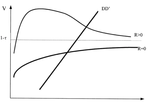
VN5(pN(12p) ((12t)N1R)2R(12(12p) )) /N . (3) This is no longer necessarily monotonic and Fig. 1 depicts the possible shapes of the relationship between sales and expected value, both for a regular draw (with
R50) and a rollover draw (R.0). V(.) always asymptotes towards 12t, but for
R.0 it is from above and at a slower rate than for when R50 when it is faster
8
The existence of several prize pools is a feature of most lotto games and this suggests that they play a role in determining sales. One possible reason is that players are sensitive to variations in higher moments of the V distribution besides the variations in the mean that we emphasise here. Having prize pools that are not subject to rollovers may be a method of ensuring that sales are not dominated by intertemporal substitution in response to rollovers – that is, such prizes ensure that sales in regular weeks are not too low. Thus there are a number of identification problems that arise: as rollovers induce changes in all moments simultaneously it is likely to prove difficult to determine which moments are empirically important; when rollovers occur there is also a surge of publicity in the media that we cannot control for; and rollovers may induce intertemporal substitution which undermines our attempts to infer permanent effects on demand from observing the effects of transitory variations in price.
Fig. 1. Relationship between sales and the expected return.
and from below. In the R50 case the shape is determined by the fact that the rollover probability falls as aggregate sales rise. For R.0 this ‘peculiar economies of scale’ argument is confounded by the way in which higher sales dilute the value of the amount of the rollover from the previous draw which would imply a decreasing hyperbolic relationship between V and N. Thus the total of these two counteracting effects implies a relationship that may attain a maximum for some finite N but for sufficiently large R will be monotonically decreasing and the dilution effect eventually dominates the returns to scale effect. Notice that V is always higher in rollover draws than in regular draws, irrespective of the level of sales. Thus, it is impossible to arbitrage away the differences in V no matter what the variation in sales. This implies that there will always be some random variation in V arising from rollovers. It is, indeed, theoretically possible for the expected value to exceed unity, the cost of a ticket, so the net expected return becomes positive.
We superimpose an aggregate demand function in Fig. 1 and this illustrates why it is unlikely that the expected return would never be greater than the cost of a ticket since it would require a low level of demand in a draw with a large jackpot accumulated from previous rollovers.
The structural background to the demand curve is not spelled out since participating in an unfair bet is clearly at odds with conventional expected utility theory. One generalisation of conventional expected utility theory would be that individuals are risk averse, and so would normally reject such unfair bets, but that participating in the lottery generates some positive non-pecuniary effect on well-being. Conlisk (1993) shows that this, unlike other extensions of expected
utility theory, is consistent with lotto participation across the whole of the income distribution, and with repeated participation at low levels which seem to characterise the game.
This rationalisation of play is consistent with play being determined by a reservation expected value. That is, suppose that individual preferences can be
* * * *
characterised by a vector Vi 5hV ,V , . . . ,V , . . .i 1 i 2 it j of reservation expected
* *
values so that i will buy exactly t tickets if Vit,V,Vit11, where V is the * expected value corresponding to a particular draw. One might expect that Vit5
*
V (t ,Z ) where Z is a vector of characteristics of individual i and t is the numberi i i i
*
of tickets such that ≠V /it ≠ti,0 reflecting the possibility that there may be some fixed transactions costs to purchasing a ticket, perhaps because of stigma, and / or the possibility that diminishing returns sets in – i.e. the non-pecuniary return to owning a lottery ticket falls at the margin as the number purchased rises. Z mayi
contain characteristics such as gender, age and income. For example, one might expect that the reservation V schedule would shift upwards as income rises if this non-pecuniary benefit is a normal good and / or if there is diminishing absolute risk aversion. We would also expect the reservation levels of expected value to depend on some unobservable characteristics that are distributed across the population.
If we want to make welfare inferences we need to specify a degree of risk aversion. The nature of the lotto game is that the minimum stake is small and participants usually stake a relatively small amount, often the minimum possible. Moreover, the expected gains are very small relative to individual incomes
9
because the jackpot probability is extremely small. Thus it seems reasonable that over such a narrow range of expected gains and losses around the existing level of wealth that preferences will be locally approximately linear. That is, at least for the vast majority of players, it seems reasonable to assume local risk neutrality. Note that risk neutrality implies that the only reason why play rises in a rollover is that the expected value rises even though higher moments of the prize distribution also change. Moreover, it implies that participation requires that the lowest reservation level of V exceeds 12t to make participation optimal.
3. Data
10
Our data relates to the UK National Lottery that started in November 1994. The UK game is a variety of the common 6 / 49 design (six balls are drawn from
9
Evidence from a survey of 2029 individuals conducted by National Opinion Polls in 1995 for the Consumers’ Association indicated widespread ignorance of the jackpot probability but no systematic tendency towards optimism or pessimism.
10
While the Family Expenditure Survey has begun to collect information on lottery ticket expenditure which distinguishes the National Lottery lotto on-line draw from scratchcards and from other lotteries (which are charitable non-pari-mutuel games and are empirically unimportant) in-sufficient data has yet to accumulate to allow econometric modelling.
49 without replacement) with a draw offering tax-free cash prizes which are proportionate to the sales revenue. Forty-five percent of the revenue is returned as prizes: all three ball matches are paid £10; 52% of the remainder is reserved for the jackpot six-ball match; and the rest split into prize pools offering smaller prizes. The chance of matching all six balls is approximately 1 in 14 million and, since sales have typically exceeded £65 million per draw, the implied mean
11
number of jackpot winners is 4.3 a week. All UK prizes are paid tax-free, as cash, in full, and immediately. With sales of approximately £65 million and a 1 in 57 chance of winning £10 the three-ball prize pool will average £11 million, leaving approximately £10 million for a jackpot. In the time series data, when a single rollover of this size occurs it typically seems to generate a jackpot of close to £20 million and an increase in sales of around 20%. A double rollover generates a jackpot of close to £40 million and, on the two occasions this has happened, this seems to have added more than 50% to sales.
The data is made up from pooling five sample surveys of approximately 1800 individuals each collected by National Opinion Polls on behalf of the Office of the
12
National Lottery (OFLOT), the industry regulator. One of these surveys, by chance, coincided with a ‘double’ rollover (that is, the jackpot from the two preceding draws had not been won). Thus approximately 20% of our sample is obtained from a survey where the expected value was exogenously higher. The final sample contained 9077 observations, some 1795 of which were drawn from
13
the double rollover survey.
Table 1 gives the means broken down into participants and non-participants, and into rollover participants and regular draw participants. The data all relates to the individual rather than the household. Only individuals aged 16 (the legal minimum for purchasing a lottery ticket) and over were interviewed. There are some obvious differences between the regular draws and the double rollover draw. The expected value of a ticket is determined by the level of sales and the size of any rollover: the average V for the regular draws was 0.45 compared with 0.62 for the double rollover – a 38% increase.
The proportion of individuals who participated in the regular weeks was 63.3%, while the proportion that participated in the double rollover week was 72.9%. The extent of participation also changes quite markedly in rollover draws, as well as the level of participation. The respective average levels of expenditure was £1.52
11
If there is no conscious selection the standard deviation around this mean would be 2.11. The importance of conscious selection is evidenced in two draws where the number of jackpot winners exceeded 50.
12
These surveys corresponded to the draws in weeks 35, 43, 60, 65, and 78 where the first draw of the National Lottery was the second week of November 1994. More comprehensive descriptions of the data can be found in Annex 3 of Office of the National Lottery (1995), (1996).
13
We dropped all observations where the level of participation exceeded £49 in the survey week (some 27 observations, one of which was top coded at £999), although the results are not sensitive to this.
Table 1
Summary statistics
Variable Non-participants Participants Rollover draw Regular draw (n53162) (n55915) participants participants (n51308) (n54607) Expenditure 0 2.562 3.114 2.406 Participation 0 1 0.633 0.729 Male 0.428 0.469 0.471 0.468 Married 0.504 0.667 0.640 0.675 Single 0.307 0.186 0.222 0.176 Separated 0.016 0.146 0.138 0.149 Left school,15 0.188 0.167 0.170 0.155 Left school 15 0.149 0.246 0.253 0.221 Left school 16 0.233 0.296 0.297 0.290 Left school 17–18 0.137 0.148 0.144 0.162 Left school 191 0.169 0.102 0.097 0.119 Age 16–18 0.102 0.036 0.045 0.033 Age 19–24 0.108 0.076 0.093 0.071 Age 25–34 0.149 0.206 0.217 0.203 Age 35–44 0.134 0.171 0.152 0.177 Age 45–54 0.132 0.189 0.179 0.192 Age 55–64 0.102 0.132 0.130 0.133 Age 651 0.273 0.190 0.184 0.192 Income,£4500 0.106 0.075 0.069 0.077 Income £4500–£9500 0.122 0.144 0.141 0.145 Income £9500–£15,500 0.077 0.108 0.107 0.108 Income £15,500–£25,000 0.066 0.177 0.112 0.119 Income £25,0001 0.101 0.105 0.103 0.105 Income refused 0.529 0.452 0.476 0.447 Employee 0.322 0.470 0.459 0.473 Self employed 0.042 0.044 0.045 0.043 Student 0.123 0.042 0.054 0.038 Retired 0.299 0.227 0.226 0.228 Unemployed / non-participant 0.213 0.216 0.217 0.218
and £2.27 – an increase of 49%. The means, conditional on participating, are £2.40 and £3.11. The data appears to match the aggregate sales data reasonably well. Grossing the average figures from the complete samples up by a factor of 46 million (the number of 161 in the population) we predict average aggregate sales of £69 million over the four regular draws which compares with actual average sales of £69 million, and £104 million in the double rollover compared with the
14
actual £128 million.
14
The wording of the questions suggests that our data excludes, or at least under-records, ‘syndicates’ where a number of people agree to purchase tickets collectively, perhaps to spread risk. There is no published information concerning the importance of these but it has been suggested to us that syndicates often accumulate small winnings and spend those winnings during rollover weeks. This would explain our under-recording of sales in the rollover draw.
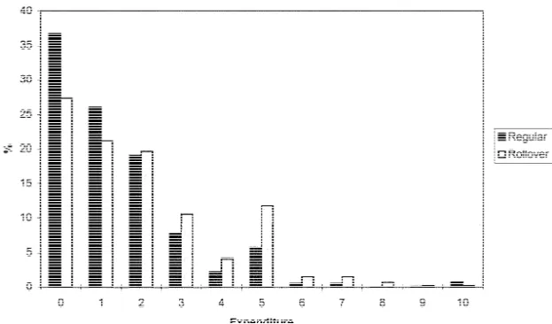
Fig. 2. Expenditure distributions in rollover and regular weeks.
The distribution of expenditure is given in Fig. 2. The typical player in regular weeks spends a modest £1 or £2, while in rollover weeks there is a much stronger tendency to spend £5 or even £10 (each lottery ‘ticket’ has space for the purchase
15
of five chances). There are also some differences across individuals with different characteristics. Men are more likely to play, and buy much more when they do play, than women. We also find that play peaks at middle age and the extent to which young people play seems quite modest – participation by the youngest group is just 39.4% compared to 56.7% for the older groups. Employed individuals have greater average expenditure than individuals of other employment statuses for both men and women. Married individuals may have greater opportunities to syndicate (with the spouse) but both single men and single women have much lower average expenditure (£1.54 and £1.06, respectively) than married men and women (£2.29 and £1.60, respectively).
Unfortunately, income is recorded in our data in grouped format and contains many missing values. Since we have a particular interest in the effect of income on demand we compute predicted values for incomes based on the observed characteristics of individuals in our data: that is we estimate the relationship between a set of characteristics, x , and income in some other datasets (we use thei
1995 / 6 Family Resources Survey where x includes age, age squared, educationi
levels, region, and gender) and use the estimated coefficients to predict incomes for the OFLOT sample given their observed values of the same x variables.
15
This has since been revised to space for seven. The proportion spending more than £10 is less than 1% and the proportion spending more than £49 is 0.12%.
Arellano and Meghir (1992) apply this idea of matching ‘complementary’ data in order to splice a variable from one source into another where the variable is missing. Here the problem is less acute since the relevant variable is grouped
16
rather than missing in the dataset of interest and we exploit this additional information in the estimation methodology. Moreover, since we are interested in uncovering the income elasticity it is convenient to have a continuous income measure. Thus we group the gross weekly individual income data in the FRS into annual income bands as defined by the OFLOT data and estimate an equation for income from this grouped data to allow us to predict income as a continuous variable. The equation is estimated as a grouped dependent variable problem, precisely as in Stewart (1983), and the results are reported in Appendix A. The estimates are used to predict the income levels of observations in the OFLOT data
17
using their recorded x’s and conditioning on their observed income band.
4. Estimation and results
The structure of our model has demand determined by a comparison of expected values with reservation levels of expected values. However, the expected value of tickets in any draw will itself depend on market sales and the level of any rollover. Our theory suggested that at high levels of sales the expected value will not be
18
very sensitive to the level of sales because the expected value asymptotes to 0.45 as sales rise. Since sales typically have been very high, the variance around this level of just below 0.45, excluding rollover draws, is very small. Thus we are essentially observing demand at just two points: a high price corresponding to
V50.45 and a lower one corresponding to the rollover draw with V50.63 (obtained by inserting the actual level of aggregate sales and the rollover size into expression (2)). Thus we are effectively comparing the means across these two samples but we need to partial out the effects of other factors that also change
19
between the two samples. That is, our results on price rely on essentially two observations: the mean of the samples when there were regular draws, compared to
16
Although almost half of the sample do have the missing code recorded for the income question. 17
For OFLOT observations where the income is coded as missing we use the unconditional expectation.
18
That is, 45% of sales revenue were returned in prizes. The operator, Camelot PLC, is obliged to return 50% of its sales revenue from both the on-line draw and its scratchcards so it seems that the on-line draw is being used to cross-subsidise the scratchcards.
19
Moreover, as we suggested earlier, a rollover cannot be used as a natural experiment since there is no control group: a rollover will engender some intertemporal substitution as well as some publicity which is largely unobservable (to the researcher). Thus we may be overestimating the elasticity of sales with respect to V. However, the result here is close to that in Farrell et al. (1997) which was obtained from time series data where there are just two double rollovers and 18 single rollovers. This suggests that non-linearities may not be important and that publicity that is particularly pronounced in double rollovers may not be affecting behaviour very much.
the mean when there was a (double) rollover. This implies that there is little point
20
in investigating sensitivity to functional form and we treat the local linearity assumption as a maintained hypothesis.
The appropriate econometric framework to adopt for this problem is unclear. One might be tempted to follow Scott and Garen (1994) and use a specification where demand is determined by comparing reservation prices with the market price. In this context, the comparison would be the current V (strictly speaking a rational expectation of the level of V that will reign for the current week’s draw
21
when it is made at the end of the week ) with an individual specific vector of *
reservation levels, V , indicating the expected value that would induce one to justit
buy the tth ticket. Abstracting from the discrete nature of the dependent variable, but not its non-negative nature, we can write demand as
2 * 9 t 5x b 1u , u |N(0,s ). i i i i u * * ti if ti .0, ti5
H
0 if t*#0. (4) iThis is a Tobit specification that Scott and Garen (1994) apply to their US scratchcard data. However, the Tobit model may be unattractive because of its sensitivity to the assumption of normality of the unobservable heterogeneity. In particular, heteroscedasticity can be expected to be a problem in microdata and
22
estimates of the Tobit model are thought to be quite sensitive to the problem
23
relative to Probit or Logit.
24
Scott and Garen (1994) compare the estimates from a Tobit model, where the
20
Unfortunately, OFLOT did not manage to have any further survey fieldwork that coincided with a (single) rollover week prior to the game design changing significantly in early 1996 to two draws per week. This would have been useful since it would allow a further degree of freedom to test for linearity. Our work on the time series data does not, however, indicate any significant non-linearities – we found that the effect of a double rollover was consistent with its (large) expected value.
21
In fact, the majority of sales occur in the 12 hours preceding the draw after Camelot have made an announcement of an estimate of the likely jackpot size. These estimates have proved to be fairly accurate.
22
Johnston and DiNardo (1998) report Monte Carlo results where OLS has a smaller bias and a smaller variance than the Tobit under conditions of heteroskedasticity.
23
To address this issue we implemented the Censored Least Absolute Deviations (CLAD) procedure due to Powell (1984) in the manner suggested in Buchinsky (1994) and implemented in STATA code provided in Deaton (1997). The procedure applies a criterion which minimises the absolute deviations rather than the usual squared deviations criteria to yield a median (rather than mean) regression. One of the useful properties of the median is that it is preserved under monotone transformations so, unlike the mean regression, the median regression is not sensitive to censoring. The estimated parameters were very close to the Tobit results and are not reported. While we know of no formal test of Tobit vs. CLAD we found that the Tobit likelihood, evaluated at the CLAD estimates, was close to the Tobit maximum and could not be rejected by a LR test.
24
parameters of the probability of playing are strictly proportional to the parameters of the amount purchased conditional on playing, with a selection model (see Heckman, 1979). The Heckman selection model can be written as
* 9
ti 5xib 1u ,i
* 9
pi 5zig 1vi, (5)
* where the second equation is the participation equation such that pi51 if ti .0 and 0 otherwise and the covariance between u and v is given by s ±0. The
i i uv
methodology is to estimate the participation equation and use the implied hazard from this to obtain consistent estimates of the level of play conditional on
25
participation. This is a generalisation of Tobit since it does not impose proportionality in the parameters across the two equations. Thus, one reason for adopting the selection model rather than the Tobit is that the existence of fixed costs of participation undermine the reservation price rationale for the Tobit model. When more than half of the adult population are weekly players it seems unlikely that stigma can play an important role that might drive a wedge between the participation effects and the effects on play conditional on participation. Moreover, UK on-line draw tickets are readily available at more than 25,000 outlets across the country so it seems unlikely that transaction costs will be very high. Nevertheless, we find the case for applying the Heckman selection method compelling because of the strong behavioural restrictions implied by the Tobit.
However, non-parametric identification of the Heckman selection model re-quires some exclusion restriction – a variable that explains participation but can be excluded from the equation determining the level of play conditional on participa-tion (see Heckman, 1990). In fact, Scott and Garen succeed in estimating their Heckman selection model without imposing any exclusion restrictions by relying on the parametric assumptions of linearity of the tickets equation and the quite specific non-linearity of the hazard term in the x’s. We know of no other example where non-linearity alone has proved sufficient to achieve identification in practice
26
and it proved not to be possible with the data here . Thus, one difficulty we have is the inherent problem of achieving identification. Here we assume that car ownership lowers the transaction costs of participation but is not, itself, correlated with demand conditional on participation. However, we do not regard this as fully
25
This follows similar work by Mroz (1987) in the context of female labour supply. Here we estimate the model by full Maximum Likelihood rather than using two steps.
26
The problem, in practice, is that the participation equation fails to discriminate well between participants and non-participants so that predicted probabilities are clustered close to the mean participation rate where the Probit function is itself close to being linear.
satisfactory since there may well be grounds for thinking that car ownership is
27
correlated with unobservables that affect lotto demand.
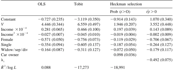
Table 2 presents the OLS, Tobit and the selection model. In addition to the expected value, we include income (predicted from our auxiliary grouped regression), and dummy variables for female, married, school leaving ages,
28
regions, and age groups.
There is a general consensus of the effects of individual characteristics across the various specifications. We find that women play less; single individuals play less; widowed, divorced and separated play less; there is some significant
Table 2
Estimates of lottery ticket purchase
OLS Tobit Heckman selection
Prob (t.O) tut.0 Constant 20.727 (0.235) 23.119 (0.350) 20.914 (0.143) 1.070 (0.340) V 4.446 (0.344) 6.559 (0.497) 1.946 (0.207) 3.552 (0.448) 24 Income310 0.281 (0.065) 0.466 (0.100) 0.197 (0.039) 0.143 (0.089) 2 24 Income 310 20.027 (0.007) 20.045 (0.010) 20.019 (0.004) 20.002 (0.009) Female 20.571 (0.050) 20.756 (0.073) 20.119 (0.029) 20.706 (0.067) Single 20.354 (0.094) 20.605 (0.137) 20.187 (0.054) 20.264 (0.127) Widow / sep / div 20.164 (0.087) 20.311 (0.127) 20.072 (0.050) 20.179 (0.117)
Car owner 0.098 (0.036)
li 20.492 (0.075)
2 ¯
R / log L 0.088 217,273 218,991
Note: The dependent variable is tickets in a specific (weekly) draw. The standard errors, corrected for using predicted income, are reported in parentheses. Heckman selection estimates are full ML estimates. Male, and married are the excluded categories. Married includes cohabitation. V, the expected value, is in £, income is recorded in £ per week. Dummy variables for 11 regions, seven school leaving ages, and six age ranges are also included. The sample is 9077 with 5915 having positive values of expenditure.
27
We would have liked to explore the sensitivity of the results to other exclusion restrictions, as Scott and Garen (1994) do, but our data contains no other plausible variables to explain participation. We plan to return to this identification when we have accumulated sufficient evidence from the UK Family Expenditure Surveys. This records expenditure over a two week period in fine detail, including lotto tickets, and is a continuous survey that is in the field all year. This offers the possibility of using time varying variables such as unanticipated weather variation. However, a second area of concern that will remain is the alleged sensitivity of the Heckman selection model to the Normality assumption. Although empirical evidence on this issue is currently sparse, Newey et al. (1990) and Stern (1996) find, albeit in small samples, that estimates that correct for selection using semi-parametric methods were not significantly different from the Heckman method. Similarly, Lanot and Walker (1998) find that union differentials are not significantly different from the Heckman results when semi-parametric methods are used in a very large sample.
28
We correct the reported standard errors for using predicted income. Note that there are no exclusion restrictions applied to our grouped regression model for predicting income so the income effects in the demand equations are identified through functional form restrictions alone.
systematic regional variation; play falls with later school leaving; and play rises
29
quickly with age, plateaus in middle age, and falls steeply in old age. The effect of the expected value is strongly positive and significant in all specifications. The effect of income is typically positive over the range of the data. The pro-portionality restriction of the Tobit is strongly rejected by the selection estimates
2
with a x of 172.2 compared to a critical value of 18.5.
Car ownership appears to be a significant determinant of participation, after controlling for the other covariates, and the selectivity term is successfully identified. As in Scott and Garen, the selection specification rejects Tobit and OLS. However, OLS (over the whole sample including the non-participants) may, nevertheless, be of some interest. OLS estimates (consistently) the effect of the change in expected value on the population mean which seems to us to be the elasticity of interest for making inferences for the population. In contrast, the
30
selection (and Tobit) results break this unconditional effect into the effect on the probability of playing and the effect conditional on playing.
The elasticities are presented in Table 3 and are all evaluated at sample means. In the Tobit and Heckman selection cases we follow MacDonald and Moffit (1980) and computed the elasticities by decomposing the unconditional means into
31
the product of the conditional mean and the probability of participation. The
Table 3
Elasticities at sample means
OLS Tobit Selection
Price Total 1.785 (0.34) 2.633 (0.50) 1.456 (0.37) Participation 2.001 (0.21) Levelut.0 0.763 (0.45) Income Total 0.267 (0.12) 0.449 (0.14) 0.132 (0.43) Participation 0.176 (0.51) Levelut.0 0.011 (0.10)
Note: Standard errors in parentheses.
29
The results are not comparable with Scott and Garen since their study relates to the ‘instant’ rather than weekly draw game. These are widely held, within the industry, to be very different products.
30
Recent work on selection correction in semi-parametric models has advocated the inclusion of power series expansions of the selection term. See, for example, Lanot and Walker (1998). Our attempt here to include a polynomial in the hazard rate into the demand equation found the quadratic term to be insignificant.
31
*
That is, ln E[t ]i 5ln(Pr(ti .0))1ln(E[tiuti.0]) so that differentiating with respect to x gives thek
elasticity of the unconditional mean with respect to x as the sum of the elasticities of participation andk
the conditional mean
* *
≠ln(E[t ])i ≠ln(E[tiuti .0]) ≠ln(Pr[ti .0])
]]]≠x 5Pr[ti*.0]]]]]≠x 1E[tiuti*.0]]]]]≠x .
32
estimated price elasticities are a little higher than the previous US studies but comparable with the UK estimates of 1.55 from the aggregate data in Farrell et al. (1997), especially the preferred selection estimates. The income elasticities are uniformly positive, but below unity, implying that lotto tickets are a normal ‘necessity’. The preferred Heckman selection estimate is particularly low. This is an important result since it is the income elasticity that determines the incidence of the tax element of the price. All of the estimates imply that the lotto tax and good causes levy is regressive, the Heckman estimates particularly so.
5. Welfare effects
We measure the welfare gain from the availability of the market for lottery tickets by the conventional consumer surplus. Our chosen linear functional form, together with risk neutrality, allows us to compute exact measures of welfare as shown in Hausman (1980) and Preston and Walker (1998). The only additional complication over the Hausman methodology is that we allow for a complication
33
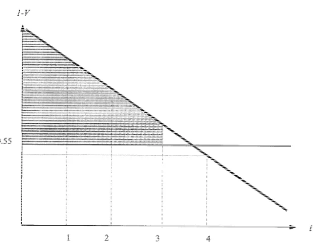
arising from the integer nature of demand. Thus, for each individual we compute the optimal integer demand, t , for a specific draw (Vi 50.45 in the case of a regular draw) using the indirect utility function corresponding to our linear demand curve and, by inverting the demand function, we can obtain the corresponding
*
reservation value of V, say V . Note, as shown in Fig. 3, that this reservation levelt
will typically be greater than 0.45 because only integer quantities are assumed to be available. Thus we do not evaluate the money metric at 0.45 but at the higher
*
reservation level and then add (Vt 20.45)t . Thus in Fig. 3, when the price isi
£0.55 the consumer will purchase three tickets and the surplus is given by the shaded area.
Table 4 presents the summary of the computations of the consumer surplus results averaging across all individuals, both participants and non-participants, for
34
each type of draw. The rollover results are larger because the consumer surplus increases with V. The Tobit results are larger because of the larger price elasticity. In order to get these figures in perspective it should be noted that the gains from a year of draws, with a typical proportion of rollovers, the estimated surplus, from the selection estimates, aggregated over the 46 million adults in the population
32
The price elasticity is the elasticity with respect to V multiplied by 2(12V ) /V since the cost of a ticket is £1 so that the ‘price’ is 12V.
33
Blow and Crawford (1997) use non-parametric revealed preference methods to show that the reservation price (which would just induce the purchase of one ticket) is approximately £1.36 on average. This surplus of about £0.80 over the net price of a ticket seems broadly consistent with the results here.
34
The samples are not random samples of the population and we use the weights provided with the data to aggregate the individual surplus measures.
Fig. 3. Demand and consumer surplus.
would be just below £1 billion per annum – the same order of magnitude as reducing the rate of income tax by 0.5%.
Table 4 shows the consumer surplus generated by the actual game design relative to not being able to play at all. One could also compute the surplus that
35
could have been generated had the game not been tied to a ‘charitable’ donation
Table 4
Summary consumer surplus measures (£ / draw)
OLS Tobit Selection Regular draw (V50.45) 0.49 0.46 0.40 Rollover draw (V50.50) 0.53 0.50 0.47 Double rollover (V50.63) 0.68 0.66 0.60
35
We do not consider the demand for scratchcards that also attract the good causes levy. This levy might be rationalised as a way of compensating charities for some loss in revenue arising from the introduction of the game. Some charities did raise funds through their own lottery games but there is little evidence to suggest that the game has had an adverse effect on private charitable giving in aggregate. For example, Banks and Tanner (1997) report no reduction in giving following the introduction of the game in late 1994.
36
for ‘good causes’ of £0.29 with each ticket. This donation raises, according to our estimates, a predicted level of revenue and a predicted loss in consumer surplus as given in Table 5. Notice that the ratio of the deadweight loss of consumer surplus to the revenue raised is large. Raising this revenue from taxing
37
this particular commodity is extremely inefficient. Finally, in Table 5 we show
38
the effects of both the 28% levy for good causes and the 12% excise duty. The results are for a typical year of draws with 42 regular draws, nine rollovers and
39
one double rollover. This seems likely to be close to what we might expect if the operator pursued marginal cost pricing. The table indicates that the corollary of the game generating considerable consumer surplus is that taxing it heavily causes a considerable loss in consumer surplus. The results are quite similar across methods which provides some reassurance as to their robustness.
Finally, although our analysis of income effects is based on rather imperfect data it is nevertheless instructive to attempt to decompose the aggregate effects presented above by income. One difficulty with this is that there is a marked
Table 5
Annual deadweight loss
Good causes 28% Good causes 28% and tax 12% OLS DWL (£b) 0.37 0.51 Revenue (£b) 1.02 1.48 DWL / R (%) 36 36 Tobit DWL (£b) 0.35 0.50 Revenue (£b) 1.00 1.50 DWL / R (%) 35 33 Selection DWL (£b) 0.34 0.48 Revenue (£b) 0.99 1.45 DWL / R (%) 34 33 36
The contract between the operator, Camelot PLC, and the UK government specifies that, on average, 28% of sales revenue be transferred to distribution funds for specific purposes such as charity, heritage, etc. In fact, the contract is more complex than this and specifies a non-linear schedule whereby the marginal tax rate rises with sales up to a maximum of 32%. Thus, our estimates are likely to underestimate the marginal deadweight loss of the levy.
37
It might be argued that there are social costs associated with the game and that part of this 28% levy is a Pigovian tax.
38
The tax rate of 12% was levied to ensure that the effect of introducing the game of tax revenue was neutral. That is, the game would draw consumer expenditure away from some goods which were untaxed and some that were highly taxed so that a rate of 12% would be broadly neutral. This need not, of course, be efficient since other goods may be less elastically demanded than lotto tickets.
39
This is what we would expect to occur using a ‘coverage rate’ of 92%, which is the average rate over the second complete year of sales, at the predicted level of sales.
lifecycle pattern of lotto behaviour as well as a well-known relationship between income and age. Individuals were ranked by the present value of the stream of incomes, predicted from the grouped regression results and discounted at a real rate of 2% per annum from aged 16 to 75. The means of the surpluses for individuals in each decile of this wealth distribution showed no systematic variation in the absolute value of the surplus with wealth, reflecting the small income elasticity from the Heckman selection estimates. The fact that the absolute value of the surplus is unrelated to wealth implies that the proportionate gains are concentrated amongst the poor. A corollary of this is that a disproportionate share of the distributional burden of the tax and good causes levy are borne by the poorest.
6. Conclusion
This paper is concerned with the demand for lottery tickets. Earlier work has looked at the responsiveness of sales to rollovers using aggregate sales data, but only one of these earlier papers attempts to derive ‘price’ elasticity. The availability of microdata here allows us to estimate both ‘price’ and income elasticities since it covers draws when there was no rollover as well as one
40
occasion when there was a (double) rollover. We find low income elasticities and high price elasticities. The former implies that taxing lotto is regressive; the latter implies that it is inefficient.
We use our estimates to speculate on the likely size of the consumer surplus arising from the availability of a market in lottery tickets. The distinctive feature of our analysis is that it is based on the ex ante gains from participation rather then
41
the ex post gains (i.e. losses). The consumer surplus is large: our best estimate is £0.41 per regular draw: with a typical proportion of rollovers this amounts to £1 billion per annum.
There are a number of deficiencies in the analysis that need to be considered. Firstly, the analysis is based on a comparison of sales in four regular draws with a single (and atypical) rollover draw. However, our time series analysis in Farrell et al. (1997) is in broad agreement with the results here.
Secondly, we ignore the possibility of intertemporal substitution. This could arise from individuals playing less in regular weeks in anticipation of rollovers in subsequent draws when the expected value would be higher despite the higher
40
Thus, we are effectively estimating the price elasticity by comparing the mean in one draw with that from the four other draws, controlling for changes in the type of person across draws.
41
Naturally the ex ante results are diametrically opposed to the ex post ones since the ex ante surplus is greatest for those that consume most who are those who, ex post, lose most.
42
level of aggregate sales. Since there are large week to week price variations we might expect this to be an important issue that could undermine the legitimacy of our current estimates for analysing policy changes. Our time series estimates imply considerable addiction which mitigates against the likelihood of widespread intertemporal substitution. Moreover, unlike several US games, the UK game has been designed in such a way that it operates quite close to its maximum expected value in regular draws. Indeed, the possibility of inter-game substitution does not exist in the UK unlike the US where it seems likely that multiple rollovers in one game attracts custom from those that usually play competing games.
Finally, our analysis presumes that choices depend only on the first moment of the return, i.e. the expected value. There are two potentially important problems that follow from this: when rollovers occur the expected return rises but there is also a considerable increase in publicity as the media debates the merits (or otherwise) of large jackpots and this might directly affect demand; and rollovers exert a large skew to the prize distribution which may have an independent effect
43
on demand. We are unable to generalise our analysis to allow for this but doubt whether design changes that might occur in practice would allow us to generalise because they are inevitably a response to developments in sales.
Acknowledgements
The National Opinion Poll surveys used here were made available to us by the Office of the National Lottery (OFLOT, the regulatory body for the UK lottery). We are grateful to Michael Richardson at OFLOT for supplying the data, and to the Economic and Social Research Council for financial support under research grant R000236821. Helpful comments were received from James Heckman, Sherwin Rosen, William Ziemba, Phillip Cook, Jonathon Simon and seminar participants at Keele, Warwick and ANU Canberra. The opinions expressed here are those of the authors alone.
Appendix A
Table 6.
42
A similar issue arises in the labour supply context. See Blundell and Walker (1986). 43
Purfield and Waldron (1996) find that skew in V is significant in their analysis of the long time series that is available for the Irish lotto game but they do not control for the mean V.
Table 6
Estimates of grouped dependent variable model
Variable Coefficient Standard error
Constant 8.111 0.442
Female 20.007 0.216
Single 20.650 0.030
Widow / sep / divorced 20.647 0.025
Left school 15 0.138 0.356 Left school 16 0.354 0.036 Left school 17 0.553 0.038 Left school 181 0.872 0.040 Age 19–25 1.199 0.442 Age 26–35 1.337 0.441 Age 36–45 1.547 0.441 Age 46–55 1.611 0.441 Age 56–65 1.425 0.441 Age 661 1.240 0.443 Log L 25526.29
Note: Region and work status dummy variables also included.
References
Arellano, M., Meghir, C., 1992. Female labour supply and on-the-job search: an empirical model estimated using complementary data sets. Review of Economic Studies 59, 537–559.
Banks, S., Tanner, S., 1997. The State of Donations: Household Gifts to Charity, 1974–96. Institute for Fiscal Studies Commentary 62, London.
DeBoer, L., 1985. Lottery taxes may be too high. Journal of Policy Analysis and Management 5, 594–596.
Blow and Crawford, 1997. A GARP method of overcoming new goods bias in price indices with an application to the national lottery, UCL DP 97 / 10.
Blundell, R.W., Walker, I., 1986. A lifecycle consistent model of family labour supply using cross section data. Review of Economic Studies 53, 539–558.
Buchinsky, M., 1994. Changes in the US wage structure 1963–1987: application of quantile regression. Econometrica 62, 405–458.
Clotfelter, C.T., Cook, P.J., 1989. Selling Hope: State Lotteries in America. Harvard University Press. Conlisk, J., 1993. The utility of gambling. Journal of Risk and Uncertainty 6, 255–275.
Cook, P.J., Clotfelter, C.T., 1993. The peculiar scale economies of lotto. American Economic Review 83, 634–643.
Deaton, A.S., 1997. The Analysis of Household Surveys. Johns Hopkins University Press, MD. Farrell, L., Hartley, R., Lanot, G., Walker, I., 1996. It could be you: rollovers and the demand for
lottery tickets. Working Paper 96 / 16, Keele University.
Farrell, L., Morgenroth, E., Walker, I., 1997. The long run elasticity of demand for lotto. Working Paper 97 / 04, Keele University.
Gulley, O.D., Scott Jr, F.A., 1993. The demand for wagering on state-operated lotto games. National Tax Journal 46, 13–22.
Hausman, J., 1980. Labour supply. In: Ashenfelter, O., Layard, R. (Eds.), Handbook of Labour Economics. North-Holland, Amsterdam.
Heckman, J.J., 1979. Sample selection as a specification error. Econometrica 42, 153–161. Heckman, J.J., 1990. Varieties of selection bias. American Economic Review (Papers and Proceedings)
80, 313–328.
Johnston, J., DiNardo, J., 1998. Econometric Methods. McGraw-Hill, New York.
Lanot, G., Walker, I., 1998. The union / non-union wage differentials: an application of semi-parametric methods. Journal of Econometrics 84, 327–349.
Lim, F.W., 1995. On the distribution of the lotto. ANU Working Papers in Economics and Econometrics 282.
Livernois, J., 1987. The redistributive effect of lotteries: evidence from Canada. Public Finance Quarterly 15, 339–351.
MacDonald, J., Moffit, R., 1980. The uses of Tobit analysis. Review of Economics and Statistics 62, 318–321.
Mroz, T., 1987. The sensitivity of an empirical model of married women’s hours of work to economic and statistical assumptions. Econometrica 54, 765–799.
Newey, W., Powell, J., Walker, J., 1990. Semi-parametric estimation of selection models: some empirical results. American Economic Review 80, 324–328.
Office of the National Lottery, 1995. Social Research Commissioned 31 / 1 / 95–31 / 1 / 96. OFLOT, London.
Office of the National Lottery, 1996. Social Research Commissioned 1 / 2 / 96–1 / 6 / 96. OFLOT, London.
Powell, J., 1984. Least absolute deviations estimation for the censored regression model. Journal of Econometrics 25, 303–325.
Preston, I., Walker, I., 1998. Welfare measurement in labour supply models with nonlinear budget constraints. Journal of Population Economics (in preparation).
Purfield, C., Waldron, P., 1996. Competitive interaction between the national lottery and betting shops in the Irish gambling market. Mimeo, Trinity College Dublin.
Scoggins, J.F., 1995. The lotto and expected net revenue. National Tax Journal 48, 61–70. Scott, F., Garen, J., 1994. Probability of purchase, amount of purchase, and the demographic incidence
of the lottery tax. Journal of Public Economics 54, 121–143.
Sprowls, C.R., 1970. On the terms of the New York State lottery. National Tax Journal 23, 74–82. Stern, S., 1996. Semi-parametric estimates of the supply and demand effects of disability on labour
force participation. Journal of Econometrics 71, 49–70.
Stewart, M., 1983. On least squares estimation when the dependent variable is grouped. Review of Economic Studies 50, 737–753.
Vrooman, D.H., 1976. An economic analysis of the New York State lottery. National Tax Journal December, 482–488.