Level Set Evolution Without Re-initialization: A New Variational Formulation

(1)

Level Set Evolution Without Re-initialization: A New Variational Formulation

Chunming Li

1

_{, Chenyang Xu}

2

_{, Changfeng Gui}

3

_{, and Martin D. Fox}

1

_{Department of Electrical and}

2

_{Department of Imaging}

3

_{Department of Mathematics}

Computer Engineering

and Visualization

University of Connecticut

Siemens Corporate Research

Storrs, CT 06269, USA

Princeton, NJ 08540, USA

{cmli,fox}@engr.uconn.edu

Abstract

In this paper, we present a new variational formulation for geometric active contours that forces the level set func-tion to be close to a signed distance funcfunc-tion, and therefore completely eliminates the need of the costly re-initialization procedure. Our variational formulation consists of an in-ternal energy term that penalizes the deviation of the level set function from a signed distance function, and an exter-nal energy term that drives the motion of the zero level set toward the desired image features, such as object bound-aries. The resulting evolution of the level set function is the gradient flow that minimizes the overall energy func-tional. The proposed variational level set formulation has three main advantages over the traditional level set formu-lations. First, a significantly larger time step can be used for numerically solving the evolution partial differential equa-tion, and therefore speeds up the curve evolution. Second, the level set function can be initialized with general func-tions that are more efficient to construct and easier to use in practice than the widely used signed distance function. Third, the level set evolution in our formulation can be easily implemented by simple finite difference scheme and is computationally more efficient. The proposed algorithm has been applied to both simulated and real images with promising results.

1. Introduction

In recent years, a large body of work on geometric ac-tive contours, i.e., acac-tive contours implemented via level set methods, has been proposed to address a wide range of im-age segmentation problems in imim-age processing and com-puter vision (cf. [3, 5, 7]). Level set methods were first in-troduced by Osher and Sethian [11] for capturing moving fronts. Active contours were introduced by Kass, Witkins, and Terzopoulos [1] for segmenting objects in images using dynamic curves. The existing active contour models can be

broadly classified as eitherparametric active contour mod-els or geometric active contour models according to their representation and implementation. In particular, the para-metric active contours [1, 2] are represented explicitly as parameterized curves in a Lagrangian framework, while the geometric active contours [5–7] are represented implicitly as level sets of a two-dimensional function that evolves in an Eulerian framework.

Geometric active contours are independently introduced by Caselles et al. [5] and Malladiet al.[7], respectively. These models are based on curve evolution theory [10] and level set method [17]. The basic idea is to represent con-tours as the zero level set of an implicit function defined in a higher dimension, usually referred as thelevel set function, and to evolve the level set function according to a partial dif-ferential equation (PDE). This approach presents several ad-vantages [4] over the traditional parametric active contours. First, the contours represented by the level set function may break or merge naturally during the evolution, and the topo-logical changes are thus automatically handled. Second, the level set function always remains a function on a fixed grid, which allows efficient numerical schemes.

Early geometric active contour models (cf. [5–7]) are typically derived using a Lagrangian formulation that yields a certain evolution PDE of a parametrized curve. This PDE is then converted to an evolution PDE for a level set func-tion using the related Eulerian formulafunc-tion from level set methods. As an alternative, the evolution PDE of the level set function can be directly derived from the problem of minimizing a certain energy functional defined on the level set function. This type of variational methods are known as variational level set methods [8, 9, 14].

Compared with pure PDE driven level set methods, the variational level set methods are more convenient and natural for incorporating additional information, such as region-based information [8] and shape-prior information [9], into energy functionals that are directly formulated in the level set domain, and therefore produce more robust re-sults. For examples, Chan and Vese [8] proposed an

(2)

ac-tive contour model using a variational level set formulation. By incorporating region-based information into their energy functional as an additional constraint, their model has much larger convergence range and flexible initialization. Vemuri and Chen [9] proposed another variational level set formula-tion. By incorporating shape-prior information, their model is able to perform joint image registration and segmentation. In implementing the traditional level set methods, it is numerically necessary to keep the evolving level set func-tion close to a signed distance funcfunc-tion [15, 17]. Re-initialization, a technique for periodically re-initializing the level set function to a signed distance function during the evolution, has been extensively used as a numerical rem-edy for maintaining stable curve evolution and ensuring usable results. However, as pointed out by Gomes and Faugeras [12], re-initializing the level set function is ob-viously a disagreement between the theory of the level set method and its implementation. Moreover, many proposed re-initialization schemes have an undesirable side effect of moving the zero level set away from its original location. It still remains a serious problem as when and how to apply the re-initialization [12]. So far, the re-initialization proce-dure has often been applied in an ad-hoc manner.

In this paper, we present a new variational formulation that forces the level set function to be close to a signed distance function, and therefore completely eliminates the need of the costly re-initialization procedure. Our varia-tional energy funcvaria-tional consists of an internal energy term and an external energy term, respectively. The internal en-ergy term penalizes the deviation of the level set function from a signed distance function, whereas the external en-ergy term drives the motion of the zero level set to the de-sired image features such as object boundaries. The result-ing evolution of the level set function is the gradient flow that minimizes the overall energy functional. Due to the in-ternal energy, the level set function is naturally and automat-ically kept as an approximate signed distance function dur-ing the evolution. Therefore, the re-initialization procedure is completely eliminated. The proposed variational level set formulation has three main advantages over the traditional level set formulations. First, a significantly larger time step can be used for numerically solving the evolution PDE, and therefore speeds up the curve evolution. Second, the level set function could be initialized as functions that are com-putationally more efficient to generate than the signed dis-tance function. Third, the proposed level set evolution can be implemented using simple finite difference scheme, in-stead of complex upwind scheme as in traditional level set formulations. The proposed algorithm has been applied to both simulated and real images with promising results. In particular it appears to perform robustly in the presence of weak boundaries.

In the following sections, we give necessary background, describe our method and its implementation, and provide experimental results that show the overall characteristics

and performance of this method.

2. Background

2.1. Traditional Level Set Methods

In level set formulation of moving fronts (or active con-tours), the fronts, denoted byC, are represented by the zero level setC(t) ={(x, y)|φ(t, x, y) = 0}of a level set func-tionφ(t, x, y). The evolution equation of the level set func-tionφcan be written in the following general form:

∂φ

∂t +F|Oφ|= 0 (1) which is called level set equation [11]. The function F is called the speed function. For image segmentation, the functionFdepends on the image data and the level set func-tionφ.

In traditional level set methods [5–7, 17], the level set functionφcan develop shocks, very sharp and/or flat shape during the evolution, which makes further computation highly inaccurate. To avoid these problems, a common nu-merical scheme is to initialize the function φas a signed distance function before the evolution, and then “reshape” (or “re-initialize”) the function φ to be a signed distance function periodically during the evolution. Indeed, the re-initialization process is crucial and cannot be avoided in us-ing traditional level set methods [4–7].

2.2. Drawbacks Associated with Re-initialization

Re-initialization has been extensively used as a numeri-cal remedy in traditional level set methods [5–7]. The stan-dard re-initialization method is to solve the following re-initialization equation

∂φ

∂t = sign(φ0)(1− |Oφ|) (2) whereφ0 is the function to be re-initialized, andsign(φ)

is the sign function. There has been copious literature on re-initialization methods [15, 16], and most of them are the variants of the above PDE-based method. Unfortunately, if φ0 is not smooth orφ0is much steeper on one side of the

interface than the other, the zero level set of the resulting functionφcan be moved incorrectly from that of the origi-nal function [4, 15, 17]. Moreover, when the level set func-tion is far away from a signed distance funcfunc-tion, these meth-ods may not be able to re-initialize the level set function to a signed distance function. In practice, the evolving level set function can deviate greatly from its value as signed dis-tance in a small number of iteration steps, especially when the time step is not chosen small enough.

So far, re-initialization has been extensively used as a nu-merical remedy for maintaining stable curve evolution and

(3)

ensuring desirable results. From the practical viewpoints, the re-initialization process can be quite complicated, ex-pensive, and have subtle side effects. Moreover, most of the level set methods are fraught with their own problems, such as when and how to re-initialize the level set function to a signed distance function [12]. There is no simple answer that applies generally [15] to date. The variational level set formulation proposed in this paper can be easily imple-mented by simple finite difference scheme, without the need of re-initialization.

3. Variational Level Set Formulation of Curve

Evolution Without Re-initialization

3.1. General Variational Level Set Formulation with

Penalizing Energy

As discussed before, it is crucial to keep the evolv-ing level set function as an approximate signed distance function during the evolution, especially in a neighbor-hood around the zero level set. It is well known that a signed distance function must satisfy a desirable property of

|Oφ|= 1. Conversely, any functionφsatisfying|Oφ|= 1

is the signed distance function plus a constant [19]. Natu-rally, we propose the following integral

P(φ) = Z Ω 1 2(|Oφ| −1) 2_dxdy ₍₃₎

as a metric to characterize how close a function φis to a signed distance function inΩ⊂ <2_{. This metric will play a}

key role in our variational level set formulation.

With the above defined functionalP(φ), we propose the following variational formulation

E(φ) =µP(φ) +Em(φ) (4)

whereµ >0is a parameter controlling the effect of penal-izing the deviation ofφfrom a signed distance function, and

Em(φ)is a certain energy that would drive the motion of the

zero level curve ofφ.

In this paper, we denote by∂E

∂φthe Gateaux derivative (or

first variation) [18] of the functionalE, and the following evolution equation:

∂φ ∂t =−

∂E

∂φ (5)

is thegradient flow [18] that minimizes the functional E. For a particular functionalE(φ)defined explicitly in terms ofφ, the Gateaux derivative can be computed and expressed in terms of the functionφand its derivatives [18].

We will focus on applying the variational formulation in (4) to active contours for image segmentation, so that the zero level curve ofφcan evolve to the desired features in the image. For this purpose, the energyEmwill be defined

as a functional that depends on image data (see below), and therefore we call it theexternal energy. Accordingly, the energyP(φ)is called theinternal energyof the functionφ, since it is a function ofφonly.

During the evolution ofφaccording to the gradient flow (5) that minimizes the functional (4), the zero level curve will be moved by the external energyEm. Meanwhile, due

to the penalizing effect of the internal energy, the evolv-ing functionφwill be automatically maintained as an ap-proximate signed distance function during the evolution ac-cording to the evolution (5). Therefore the re-initialization procedure is completely eliminated in the proposed formu-lation. This concept is demonstrated further in the context of active contours next.

3.2. Variational Level Set Formulation of Active

Contours Without Re-initialization

In image segmentation, active contours are dynamic curves that moves toward the object boundaries. To achieve this goal, we explicitly define an external energy that can move the zero level curve toward the object boundaries. Let Ibe an image, andgbe theedge indicator functiondefined by

g= 1

1 +|OGσ∗I|2,

whereGσis the Gaussian kernel with standard deviationσ.

We define an external energy for a functionφ(x, y)as below

Eg,λ,ν(φ) =λLg(φ) +νAg(φ) (6)

whereλ >0andνare constants, and the termsLg(φ)and

Ag(φ)are defined by Lg(φ) = Z Ω gδ(φ)|Oφ|dxdy (7) and Ag(φ) = Z Ω gH(−φ)dxdy, (8) respectively, where δis the univariate Dirac function, and H is the Heaviside function.

Now, we define the following total energy functional

E(φ) =µP(φ) +Eg,λ,ν(φ) (9)

The external energyEg,λ,ν drives the zero level set toward

the object boundaries, while the internal energyµP(φ) pe-nalizes the deviation of φfrom a signed distance function during its evolution.

To understand the geometric meaning of the energy

Lg(φ), we suppose that the zero level set of φ can be

represented by a differentiable parameterized curve C(p), p ∈ [0,1]. It is well known [9] that the energy functional

Lg(φ) in (7) computes the length of the zero level curve

(4)

0 10 20 30 40 50 600 20 40 60 −10 −5 0 5 10 15 20 25 30 35 40 0 10 20 30 40 50 600 20 40 60 −15 −10 −5 0 5 10 15 20 25 30 35 0 10 20 30 40 50 600 20 40 60 −15 −10 −5 0 5 10 15 20 25 30 35 0 10 20 30 40 50 600 20 40 60 −15 −10 −5 0 5 10 15 20 25 30 35

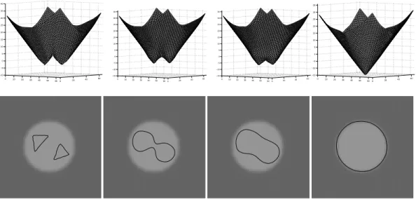
Figure 1. Evolution of level set functionφ. Row 1: the evolution of the level set functionφ. Row 2: the evolution of the zero level curve of the corresponding level set functionφin Row 1.

energy functionalAg(φ)in (8) is introduced to speed up

curve evolution. Note that, when the function g is con-stant1, the energy functional in (8) is the area of the region

Ω−

φ = {(x, y)|φ(x, y) < 0} [17]. The energy functional

Ag(φ)in (8) can be viewed as the weighted area ofΩ−_φ. The

coefficientν ofAgcan be positive or negative, depending

on the relative position of the initial contour to the object of interest. For example, if the initial contours are placed out-side the object, the coefficientνin the weighted area term should take positive value, so that the contours can shrink faster. If the initial contours are placed inside the object, the coefficientνshould take negative value to speed up the expansion of the contours.

By calculus of variations [18], the Gateaux derivative (first variation) of the functionalEin (9) can be written as

∂E ∂φ = −µ[Mφ−div( Oφ |Oφ|)] −λδ(φ)div(g Oφ |Oφ|)−νgδ(φ)

whereMis the Laplacian operator. Therefore, the functionφ that minimizes this functional satisfies the Euler-Lagrange equation ∂E

∂φ = 0. The steepest descent process for

mini-mization of the functionalEis the following gradient flow: ∂φ ∂t =µ[Mφ−div( Oφ |Oφ|)] +λδ(φ)div(g Oφ |Oφ|) +νgδ(φ) (10) This gradient flow is the evolution equation of the level set function in the proposed method.

The second and the third term in the right hand side of (10) correspond to the gradient flows of the energy

func-tionalλLg(φ)andνAg(φ), respectively, and are

responsi-ble of driving the zero level curve towards the object bound-aries. To explain the effect of the first term, which is as-sociated to the internal energy µP(φ), we notice that the gradient flow

Mφ−div( Oφ

|Oφ|) = div[(1−

1

|∇φ|)∇φ]

has the factor (1− 1

|∇φ|)as diffusion rate. If|∇φ| > 1, the diffusion rate is positive and the effect of this term is the usual diffusion, i.e. makingφmore even and therefore reduce the gradient|∇φ|. If|∇φ| <1, the term has effect of reverse diffusion and therefore increase the gradient.

We use an image of a circular object, as shown in Fig. 1, to show the evolution ofφaccording to Eq. (10). In Fig. 1, the first figure in the upper row shows the initial level set function, and its zero level curve is plotted in first figure in the lower row. The upper row shows the evolution of the level set functionφ, and the lower row shows the cor-responding zero level curve ofφ. The fourth column is the converged result of the evolution. As we can see from this figure, during the evolution, the evolving level set function φis maintained very close to a signed distance function.

4. Implementation

4.1. Numerical Scheme

In practice, the Dirac function δ(x) in (10) is slightly smoothed as the following functionδε(x)defined by:

δε(x) = ½ 0, |x|> ε 1 2ε[1 + cos(πxε )], |x| ≤ε. (11)

(5)

We use the regularized Dirac δε(x)withε = 1.5, for all

the experiments in this paper. Because of the diffusion term introduced by our penalizing energy, we no longer need the upwind scheme [4] as in the traditional level set methods. Instead, all the spatial partial derivatives ∂φ_∂x and ∂φ_∂y are approximated by the central difference, and the temporal partial derivative ∂φ_∂t is approximated by the forward differ-ence. The approximation of (10) by the above difference scheme can be simply written as

φk_i,j+1−φk i,j

τ =L(φ

k

i,j) (12)

whereL(φi,j)is the approximation of the right hand side in

(10) by the above spatial difference scheme. The difference equation (12) can be expressed as the following iteration:

φk_i,j+1=φki,j+τ L(φki,j) (13)

4.2. Selection of Time Step

In implementing the proposed level set method, the time stepτ can be chosen significantly larger than the time step used in the traditional level set methods. We have tried a large range of the time stepτ in our experiments, from0.1

to100.0. For example, we have usedτ = 50.0 andµ = 0.004for the image in Fig. 1, and the curve evolution only takes40iterations, while the curve converge to the object boundary precisely.

A natural question is: what is the range of the time stepτ for which the iteration (13) is stable? From our experiments, we have found that the time step τ and the coefficient µ must satisfyτ µ < 1

4 in the difference scheme described in

Section 4.1, in order to maintain stable level set evolution. Using larger time step can speed up the evolution, but may cause error in the boundary location if the time step is chosen too large. There is a tradeoff between choosing larger time step and accuracy in boundary location. Usually, we useτ≤10.0for the most images.

4.3. Flexible Initialization of Level Set Function

In traditional level set methods, it is necessary to initial-ize the level set function φas a signed distance function φ0. If the initial level set function is significantly different

from a signed distance function, then the re-initialization schemes are not able to re-initialize the function to a signed distance function. In our formulation, not only the re-initialization procedure is completely eliminated, but also the level set functionφis no longer required to be initial-ized as a signed distance function.

Here, we propose the following functions as the initial functionφ0. Let Ω0 be a subset in the image domainΩ,

and∂Ω0 be all the points on the boundaries ofΩ0, which

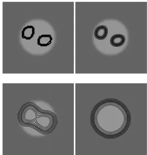
Figure 2. Isocontours plot of the level set functionφ, using the proposed initial functionφ0 defined by (14) withρ = 6. Seven

isocontours are plotted at the levels -3, -2, -1, 0, 1, 2, and 3, with the dark thicker curves being the zero level curves.

can be efficiently identified by some simple morphological operations. Then, the initial functionφ0is defined as

φ0(x, y) =      −ρ, (x, y)∈Ω0−∂Ω0 0 (x, y)∈∂Ω0 ρ Ω−Ω0 (14)

whereρ > 0is a constant. We suggest to chooseρlarger than2ε, whereεis the width in the definition of the regu-larized Dirac functionδεin (11).

Unlike signed distance functions, which are computed from a contour, the proposed initial level set functions are computed from an arbitrary regionΩ0in the image domain

Ω. Such region-based initialization of level set function is not only computationally efficient, but also allows for flex-ible applications in some situations. For example, if the re-gions of interest can be roughly and automatically obtained in some way, such as thresholding, then we can use these roughly obtained regions as the regionΩ0 to construct the

initial level set functionφ0. Then, the initial level set

func-tion will evolve stably according to the evolufunc-tion equafunc-tion , with its zero level curve converged to the exact boundary of the region of interest. To demonstrate the effectiveness of the proposed initialization scheme, we apply the proposed initialization and evolution model for the same image in Fig. 1. The initial level set function φ0 is constructed as

a function defined by (14) withρ = 6andΩ0 containing

two separate regions. By definition, this initial functionφ only takes three values: -6, 0, and 6, and its iscontours are

(6)

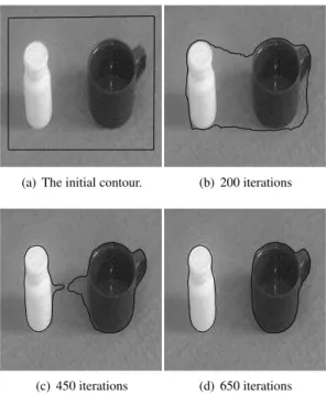
(a) The initial contour. (b) 200 iterations

(c) 450 iterations (d) 650 iterations

Figure 3. Result for a real image of a cup and a bottle, withλ= 5.0,µ= 0.04,ν= 3.0, and time stepτ = 5.0.

plotted in the first figure in Fig. 2. The evolution ofφfrom its initial valuesφ0is shown in Fig. 2 by plotting the level

curves at seven levels -3, -2, -1, 0, 1, 2, and 3, with the dark thicker ones as the zero level curves (the ones in the middle of the seven isocontours). As clearly seen in this figure, the level set function eventually become very close to a signed distance function, whose isocontours at these seven levels are almost equally spaced, with the distance between two adjacent isocontours very close to 1.

Note that this kind of initial functionφ0significantly

de-viates from a signed distance function. During the evolu-tion, the level set function φmay not be able to keep its profile globally as an approximate signed distance function in the entire image domain. But the evolution based on the proposed penalizing diffusion still maintains the level set functionφas an approximate signed distance function near the zero level set. Indeed, we have demonstrated this desir-able property in the example shown in Fig. 2.

5. Experimental Results

The proposed variational level set method has been ap-plied to a variety of synthetic and real images in different modalities. In all the experimental results shown in this sec-tion, the level set functions are initialized as the functionφ0

defined by (14) withρ= 6and some regionsΩ0.

For example, Fig. 3 shows the result on a 100×200 -pixel image of a bottle and a cup. The initial level setφ0

Figure 4. Result for a real microscope cell image, withλ = 5.0, µ= 0.04,ν= 1.5, and time stepτ= 5.0.

is computed from the region enclosed by the quadrilateral enclosing, as shown in Fig. 3(a). For this image, we used the parametersλ= 5.0,µ= 0.04,ν = 3.0, and time step τ = 5.0, which is significantly larger than the time step used for traditional level set methods. The curve evolution takes 650 iterations.

Fig. 4 shows the evolution of the contour on a64×80 -pixel microscope image of two cells. As we can see, some parts of the boundaries of the two cells are quite blurry. We use this image to demonstrate the robustness of our method in the presence of weak object boundaries. We used the re-gion below the straight line, shown in Fig. 4(a), as the rere-gion

Ω0for computing the initial level set functionφ0. As shown

in Fig. 4, this initial straight line successfully evolved to the object boundaries, and the shape of them are recovered very well. This result demonstrates desirable performance of our method in extracting weak object boundaries, which is usually very difficult for the traditional level set methods to apply [8].

Our method has also been applied to ultrasound images. Ultrasound images are notorious for the speckle noise and low signal-to-noise ratio, and therefore is very difficult to apply traditional methods to extract the object boundaries. Fig. 5 shows the results of our method for a 110×130 -pixel ultrasound image of carotid artery. The boundary of the carotid artery was successfully extracted by our method despite the presence of strong noise.

(7)

Figure 5. Result for an ultrasound image of carotid artery, with λ= 6.0,µ= 0.1,ν=−3.0, and time stepτ= 2.0.

6. Conclusions

In this paper, we present a new variational level set formulation that completely eliminates the need of the re-initialization. The proposed level set method can be easily implemented by using simple finite difference scheme and is computationally more efficient than the traditional level set methods. In our method, significantly larger time step can be used to speed up the curve evolution, while main-taining stable evolution of the level set function. Moreover, the level set function is no longer required to be initialized as a signed distance function. We propose a region-based initialization of level set function, which is not only com-putationally more efficient than computing signed distance function, but also allows for more flexible applications. We demonstrate the performance of the proposed algorithm us-ing both simulated and real images, and in particular its robustness to the presence of weak boundaries and strong noise.

References

[1] M. Kass, A. Witkin, and D. Terzopoulos, “Snakes: active con-tour models”,Int’l J. Comp. Vis., vol. 1, pp. 321-331, 1987. [2] C. Xu and J. Prince, “Snakes, shapes, and gradient vector

flow”,IEEE Trans. Imag. Proc., vol. 7, pp. 359-369, 1998.

[3] X. Han, C. Xu and J. Prince, “A topology preserving level set method for geometric deformable models”,IEEE Trans. Patt. Anal. Mach. Intell., vol. 25, pp. 755-768, 2003.

[4] J. A. Sethian,Level set methods and fast marching methods, Cambridge: Cambridge University Press, 1999.

[5] V. Caselles, F. Catte, T. Coll, and F. Dibos, “A geomet-ric model for active contours in image processing”,Numer. Math., vol. 66, pp. 1-31, 1993.

[6] V. Caselles, R. Kimmel, and G. Sapiro, “Geodesic active con-tours”,Int’l J. Comp. Vis., vol. 22, pp. 61-79, 1997.

[7] R. Malladi, J. A. Sethian, and B. C. Vemuri, “Shape modeling with front propagation: a level set approach”, IEEE Trans. Patt. Anal. Mach. Intell., vol. 17, pp. 158-175, 1995. [8] T. Chan and L. Vese, “Active contours without edges”,IEEE

Trans. Imag. Proc., vol. 10, pp. 266-277, 2001.

[9] B. Vemuri and Y. Chen, “Joint image registration and segmen-tation”,Geometric Level Set Methods in Imaging, Vision, and Graphics, Springer, pp. 251-269, 2003.

[10] B. B. Kimia, A. Tannenbaum, and S. Zucker, “Shapes, shocks, and deformations I: the components of two-dimensional shape and the reaction-diffusion space”,Int’l J. Comp. Vis., vol. 15, pp. 189-224, 1995.

[11] S. Osher, J. A. Sethian, “Fronts propagating with curvature-dependent speed: algorithms based on Hamilton-Jacobi for-mulations”,J. Comp. Phys., vol. 79, pp. 12-49, 1988. [12] J. Gomes and O. Faugeras, “Reconciling distance functions

and Level Sets”,J. Visiual Communic. and Imag. Representa-tion, vol. 11, pp. 209-223, 2000.

[13] M. Sussman, P. Smereka, and S. Osher, “A level set method for momputing solutions to incompressible two-phase flow”, J. Comp. Phys., vol. 114, pp. 146-159, 1994.

[14] H. Zhao, T. Chan, B. Merriman, and S. Osher, “A variational level set approach to multiphase motion”,J. Comp. Phys., vol. 127, pp. 179-195, 1996.

[15] D. Peng, B. Merriman, S. Osher, H. Zhao, and M. Kang, “A PDE-based fast local level set method”,J. Comp. Phys., vol. 155, pp. 410-438, 1999.

[16] M. Sussman and E. Fatemi “An efficient, interface-preserving level set redistancing algorithm and its application to interfacial incompressible fluid flow”,SIAM J. Sci. Comp., vol. 20, pp. 1165-1191, 1999.

[17] S. Osher and R. Fedkiw, Level Set Methods and Dynamic Implicit Surfaces, Springer-Verlag, New York, 2002. [18] L. EvansPartial Differential Equations, Providence:

Ameri-can Mathematical Society, 1998.

[19] V. I. Arnold,Geometrical Methods in the Theory of Ordinary Differential Equations, New York: Springer-Verlag, 1983.

Level Set Evolution Without Re-initialization: A New Variational Formulation