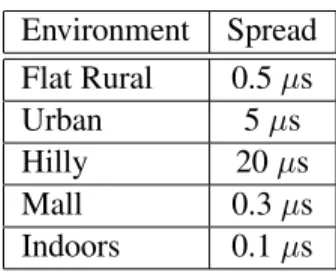
Environment Spread Flat Rural 0.5µs Urban 5µs Hilly 20µs Mall 0.3µs Indoors 0.1µs
Table 3.1: Typical delay spreads for various environments.
If W > τ1ds, then the fading is said to be frequency selective, and h(t;τ) can no longer be replaced by a
multiplication by the flat fading processE(t)as in (3.12). The goal of this section is to study how the channel
model should be modified to account for frequency selectivity.
3.5.1 CORRELATION MODELS FOR FREQUENCY SELECTIVE FADING
Recall that time-varying impulse response is given by h(t;τ) =X
n
βnejφn(t) δ(τ−τn) (3.88)
where the phase processφn(t)evolves as:
φn(t)≈ϕn+ 2πνnt
=ϕn+ 2πνmaxtcosθn
(3.89) with the phases{ϕn}being i.i.d. Unif[−π, π](see Assumption 3.2 and (3.14)). We can rewrite (3.88) as
h(t;τ) =X n
βnejϕn ej2πνntδ(τ −τn) (3.90)
Before we develop a stochastic model forh(t;τ), we introduce two additional equivalent represensentations
of the time-varying channel [Bel63].
Definition 3.11. For a channel with impulse responseh(t;τ), thetime-varying transfer functionis given by
H(t;f) = Z h(t;τ)e−j2πf τdτ =X n βnejϕn ej2π(νnt−f τn) (3.91)
and thedelay-Doppler spreading functionis given by C(ν;τ) = Z h(t;τ)e−j2πνtdt . =X n βnejϕn δ(ν−νn)δ(τ−τn) (3.92) cV. V. Veeravalli, 2007 44
Statistical Characterization ofH(t;f)
In characterizing the channel stochastically, it is easiest to deal with the time-varying transfer functionH(t;f)
since it is written as a sum of complex exponentials (rather than impulses). Since H is a function of two variables, it must be modelled as a randomfield.
The contribution of then-th path toH(t;f)can be written as
ηn(t;f) =βnejϕn ej2π(νnt−f τn) (3.93)
Analogous to the result we derived earlier in the context of frequency flat fading (Result 3.2), ηn(t;f) can
easily be seen to be a zero-mean proper complex field.
The autocorrelation function (ACF) of the fieldH(t;f)can be derived in a manner similar to the way in which
we derived the ACF of the flat fading process in (3.20). In particular, we have
E[H(t1;f1)H?(t2;f2)]≈ X
n
βn2 ej2πνn(t1−t2) e−j2πτn(f1−f2). (3.94) ThusH(t;f)is approximately stationary in bothtandf, i.e., it is approximately ahomogeneousrandom field. The homogeneous autocorrelation function can then be defined as
RH(ξ;ζ) =E[H(t+ξ;f +ζ)H?(t;f)]
≈X
n
β2nej2πνnξe−j2πτnζ. (3.95) Using the fact thatνn=νmaxcosθn, we can rewrite (3.95) as
RH(ξ;ζ) =
X
n
βn2 ej2πνmaxξcosθn e−j2πτnζ (3.96) We can express the autocorrelation function RH(ξ;ζ) in terms a quantity, which is defined below, that is
analogous to the Doppler power spectrum of (3.25):
Definition 3.12. The delay-Dopplerscattering functionis given by
Ψ(ν;τ) =X n
βn2 δ(ν−νn)δ(τ−τn). (3.97)
The scattering function Ψ(ν;τ) describes the distribution of power as a function of the Doppler frequency
and delay. The discrete joint density of (3.97) can be approximated by continuous density, by considering the paths to be forming acontinuum. As mentioned earlier, the continuous model is representative of diffuse scattering. The support of the scattering function is restricted to the rectangular region[−νmax, νmax]×[0, τds].
Furthermore, the Doppler power spectrumΨ(ν)is the marginal ofΨ(ν;τ), i.e., Ψ(ν) =
Z τds 0
Ψ(ν;τ)dτ . (3.98)
Based on (3.97), we can rewrite (3.96) as RH(ξ;ζ) = Z νmax −νmax Z τds 0 Ψ(ν;τ)ej2πνξ e−j2πτ ζ dτ dν (3.99) cV. V. Veeravalli, 2007 45
We may also express the autocorrelation functionRH(ξ;ζ)in terms of a power gain density. To this end, we
generalize the angular gain densityγ(θ)to a joint density that describes the allocation of power to both angle
of arrival and delay.
Definition 3.13. The jointangle-delay gain densityγ(θ;τ)is given by γ(θ;τ) =X
n
βn2 δ(θ−θn)δ(τ −τn). (3.100)
Obviously, there is a one-one relationship between the scattering function,Ψ(ν;τ), and the angle-delay gain
densityγ(θ, τ). A straightforward change of variables argument yields
γ(θ, τ) =νmaxsinθΨ(νmaxcosθ, τ). (3.101) Based on (3.100), we can rewrite (3.96) as
RH(ξ;ζ) = Z π −π Z τds 0 γ(θ;τ)ej2πνmaxξcosθe−j2πτ ζ dτ dθ (3.102) WSSUS Model
The zero-mean proper complex field model forH(t;f)implies that the time-varying transfer function,h(t;τ),
and the delay-Doppler spreading function,C(ν;τ), are both also zero-mean proper complex fields.
The autocorrelation function ofh(t;τ)is easily shown to be E[h(t1;τ1)h?(t2;τ2)] = " X n βn2 ej2πνn(t1−t2)δ(τ1−τn) # δ(τ1−τ2) (3.103) Note thath(t;τ)is not a homogeneous random field since it is not stationary in the delay variableτ. However, it is indeed stationary in the time variable anduncorrelatedin the delay variable. The continuous path general-ization of this model forh(t;τ)is referred to as the Wide Sense Stationary Uncorrelated Scattering (WSSUS)
model, and was first studied in great detail by Bello [Bel63]. For the continuous path generalization, we can rewrite autocorrelation function in terms of the delay-Doppler scattering function:
E[h(t+ξ;τ1)h?(t;τ2)] = Z νmax −νmax Z τds 0 Ψ(ν;τ)ej2πνξ δ(τ1−τ)dτ dθ δ(τ1−τ2) (3.104)
The autocorrelation function of the delay-Doppler spreading function,C(ν;τ), is given by E[C(ν1;τ1)C?(ν2;τ2)] = " X n β2nδ(ν1−νn)δ(τ1−τn) # δ(τ1−τ2)δ(ν1−ν2). (3.105) Thus,C(ν;τ)is not stationary inνorτ, but it is uncorrelated in both variables. Note that
E[C(ν1;τ1)C?(ν2;τ2)] = Ψ(ν1;τ1)δ(τ1−τ2)δ(ν1−ν2). (3.106)
3.5.2 RAYLEIGH AND RICEAN FADING
As we did in the study of frequency flat fading, we first characterize the distribution of the time-varying transfer function for the situation where the scattering is purely diffuse, i.e., there is no specular component. The Central Limit Theorem (Result B.3) can be applied to obtain:
Result 3.10. For purely diffuse scattering,H(t;f)is well-modelled as a zero-mean, proper complex Gaussian
random field.
As a consequence, for fixedt,f, the magnitude|H(t;f)|has a Rayleigh distribution and the phase∠H(t;f)
is uniformly distributed on[−π, π]. The corresponding model forh(t;τ)is called the Gaussian WSSUS (or
GWSSUS) model.
If there is a specular component (with possibly multiple paths) in addition to the diffuse paths, then we can write the time-varying transfer function as
H(t;f) = Ns X
n=1
βnejϕn ej2π(νnt−τnf)+ ˜β Hˇ(t;f) (3.107)
whereHˇ(t;f)is a zero-mean, proper complex Gaussian, homogeneous field, and ˜ β2 = 1− N X n=Ns+1 βn2 . (3.108)
Thus,H(t;f)is a zero-mean, proper complex, homogeneous field, but is non-Gaussian. However, conditioned on ϕ1, . . . , ϕNs, H(t;f)is a proper complex, non-homogeneous field, with non-zero mean. Also, just as in the case of the flat fading processE(t), for fixedt,f, the distribution of the envelope|H(t;f)|, conditioned on
ϕ1, . . . , ϕNs, is Ricean with Rice factor given in (3.71). If there is only one specular path, the unconditional distribution of|H(t;f)|is also Ricean.
The time-varying impulse response and delay-Doppler spreading functions get modified in a similar fashion: h(t;τ) =
Ns X
n=1
βnejϕn ej2πνntδ(τ −τn) + ˜βˇh(t;τ) (3.109)
whereˇh(t;τ)is a zero-mean, GWSSUS field.
C(ν;τ) = Ns X
n=1
βnejϕn δ(ν−νn)δ(τ −τn) + ˜βCˇ(ν;τ) (3.110)
whereCˇ(ν;τ)is a zero-mean Gaussian field that is uncorrelated inνandτ.
Chapter 4
Sampled Delay-Doppler Channel
Representations
4.1 INTRODUCTION
In this chapter we develop sampled representations for the time-varying channel h(t, τ). The motivation for
such representations is that channel modeling independent of the signal space is irrelevant from a communica-tion viewpoint — an effective channelrepresentationcommensurate with signal space characteristics is what is important. To this end, a fundamental understanding of the interaction between the signal space and the channel is critical. The sampled representations developed in this chapter precisely capture such interaction in temporal and spectral dimensions. In this context, the key signal space parameters are the signaling duration T and bandwidthW, whereas the key channel parameters are the delay spread,τds, and the Doppler spread or Doppler bandwidth,Bd= 2νmax. We assume throughout this development thatT τdsandW Bd.
The channel can be selective in time and/or frequency depending on the values for T,W,τds, andBd.
Fre-quency selectivity is determined by the number of multipath components that can be resolved by the signal within the delay spread. The delay resolution is given by the signaling bandwidth: ∆τ = 1/W. The channel is said to be frequency non-selective if τds/∆τ = W 1 and frequency selective forτdsW ≥ 1. Time selectivity is determined by the number of Doppler shifts that can be resolved by the signal within the Doppler spread. The frequency resolution is given by ∆ν = 1/T. The channel is said to be time non-selective if Bd/∆ν=BdT 1and time selective forBdT ≥1. Strictly speaking, forτdsW ≥0.2andBdT ≥0.2there
is sufficient selectivity in frequency and time, respectively, and must be taken into account [SA99].
4.2 DISCRETE-TONE APPROXIMATION FOR FREQUENCY-FLAT
FADING
Recall from Section 3.4 that for frequency-flat fading, the channel input and output are related as
y(t) =E(t)x(t) (4.1)
where E(t) = Z τds 0 h(t, τ)dτ =X n βnejϕn ej2πνnt. (4.2)
It is clear from this equation thatE(t)is a linear combination of discrete tones at the Doppler frequencies of
the paths. These tones may occur at any frequency in the range[−νmax, νmax]. This detailed description ofE(t)
implicitly assumes an infinite resolution in the frequency domain, so that each path that contributes toE(t)
can be resolved in frequency. However, infinite resolution in the frequency can only be obtained by observing the processE(t)over an infinite time horizon. This is not even approximately possible since our small scale variation model is valid only over time horizons of duration Tsmall, over which the path gains, delays, and angles of arrival remain roughly constant.
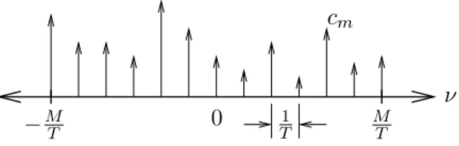
Consider modelingE(t) over the interval[0, T], whereT < Tsmall. Then, using a Fourier series expansion, we can write E(t) = ∞ X m=−∞ cme j2πmt T , t∈[0, T] (4.3) where cm = 1 T Z T 0 E(t)e−j2Tπmt dt =X n βnejϕn 1 T Z T 0 ej2πνnt e−j2Tπmt dt =X n βnejϕnejπ(νnT−m)sinc[T(νn−m/T)] (4.4)
ThusE(t)is expressed in terms of a series of equispaced Doppler frequencies. The resolution in frequency is
of course1/T, and in particular, the paths that contribute to tapcmare the ones that fall within the “sinc mask”
at Doppler frequencym/T. While the representation ofE(t)in (4.3) is more structured than the path-wise
description of given in (4.2), there are an infinite number of taps in sampled representation of (4.3). To further simplify the representation we exploit the bandlimitedness ofE(t).
As we saw in Section 3.4.5, the flat fading processE(t) is strictly bandlimited to a maximum frequency of
±νmax. We may define the two-sided bandwidth ofE(t)as:
Definition 4.1. TheDoppler bandwidthBdis defined by
Bd = 2νmax. (4.5)
The product of the time horizonTand the Doppler bandwidthBddetermines the number of degrees of freedom
(or the richness) in the flat-fading processE(t). More specifically, letM be such that
2M+ 1 =dBdTe. (4.6)
Then it is clear from (4.4) that the scattering contributes very little to tapscm, withm > M orm <−M. We
can hence approximate the infinite sum of (4.3) by the finite sum E(t)≈ M X m=−M cm e j2πmt T , t∈[0, T] (4.7)
The discrete tone approximation forE(t)given in (4.7) is described pictorially in Figure 4.1.
PSfrag replacements
ν
−MT 0 T1 MT
cm
Figure 4.1: Discrete-tone approximation for frequency-flat fading
4.2.1 STATISTICAL MODEL FOR DOPPLER TAPS
The Doppler taps of (4.4) can be rewritten as cm =
X
n
βnejϕn e−jπmsinc[T(νn−m/T)] , m=−M, . . . , M (4.8)
where we have absorbed theejνnT terms into the random phase termsejϕn without loss of generality.
Now, suppose the scattering is rich enough that the “sinc mask” corresponding to each tap captures a suffi-ciently large number of paths to apply the Central Limit Theorem. Further suppose that the scattering does not include a specular component. Then it follows thatcmhas Rayleigh statistics, i.e.,cmis zero mean proper
complex Gaussian, and that|cm|has a Rayleigh pdf. If there are one or more specular paths that contribute to
cm, thencmhas Ricean statistics. In calculating the Rice factor, the specular path gains contributing tocm of
course need to be scaled down by the “sinc mask” in (4.8).
Furthermore, using Assumption 3.2, the correlation between the taps is easily seen to be
E[cmc?k] = (−1)m−k X n βn2sinc[T(νn−m/T)]sinc[T(νn−k/T)]dθ = (−1)m−k Z νmax −νmax Ψ(ν)sinc[T(ν−m/T)]· sinc[T(ν−k/T)]dθ (4.9)
whereΨ(ν)is the Doppler power spectrum. Clearly the tapscmare not independent in general. 4.2.2 CHANNEL ESTIMATION/PREDICTION AND TIME DIVERSITY
Note that with the discrete-tone approximation, we have captured the time variations in the random process E(t)on the interval[0, T]through (deterministic) complex exponentials, and the randomness is then captured
by a finite set of random variables cm, m = −M, . . . , M. An immediate consequence of the finite Doppler
sampled representation is that the fading processE(t)can be perfectly estimated (or predicted) over the entire
interval [0, T] from a set of 2M + 1 samples of E(t) taken at distinct points in time. This has important
implications for reliable digital communications on fading channels as we discuss below.
Consider sampling the fading processE(t)in time with sampling intervalTsthat is chosen such that
Ts 1
Bd
. (4.10)
In the context of digital communications on this flat fading channel, Ts could represent the symbol period,
and condition (4.10) would then imply that the fading isslowrelative to the symbol rate (see Definition 3.10). Under condition (4.10), the fading processE(t)can be considered to be constant over intervals of durationTs,
so that we may representE(t)by the discrete-time process (sequence){Ek}, with
Ek=∆E(kTs), k= 0,1,2, . . . . (4.11)
In the following, we assume thatE(t)is aRayleighflat fading process, with the understanding that the
exten-sion to Ricean fading is straightforward. SupposeTs is such thatT =KTsfor some integerK. Then, from
(4.7) and (4.11), we obtain Ek= M X m=−M cme j2πmkTs T = M X m=−M cm e j2πmk K . (4.12)
From (4.12) it is clear that the rank of the covariance matrix of the vectorE = [E0 E1 · · · EK]is at most
equal to2M + 1. The ratio
µ=∆ 2M+ 1
K (4.13)
is a measure of variation (equivalently, the predictability) of the channel. It is also a measure of the time diversity afforded by the channel that can be exploited to counter fading at the receiver through appropriate coding. From the slow fading condition (4.10) and (4.6), we get that
µ= dBdTe
T /Ts
=dBdTse 1. (4.14)
Thus slow fading channels can provide significant time diversity only over large block lengths. On the other hand, a small value of µ implies that long-range prediction of the channel is possible, and this could be exploited to advantage at the receiver.
4.3 TAPPED DELAY LINE MODEL FOR FREQUENCY-SELECTIVE
FADING
In the previous section we exploited the finiteness of the time horizon to obtain a sampled Doppler repre-sentation of the channel. We now consider the dual problem of obtaining a sampled delay reprerepre-sentation for frequency selective channels. To do so we exploit the bandlimitedness of the signal that is transmitted on the channel. For clarity of presentation, we do not assume sampling in the Doppler domain in this section. Joint delay-Doppler sampled representations will be the subject of the next section.
Referring back to Figure 3.14, since the channel input x(t) has baseband bandwidth W/2 (and passband
bandwidthW), by the Sampling Theorem (sinc interpolation formula) we can expandx(t−τ)as:
x(t−τ) = ∞ X `=−∞ x(t−`/W) sinc[W (τ −`/W)] (4.15) cV. V. Veeravalli, 2007 52
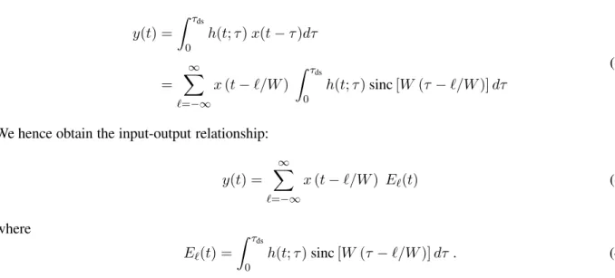
Hence, starting with (3.5), we can express the channel outputy(t)in terms ofx(t)as: y(t) = Z τds 0 h(t;τ)x(t−τ)dτ = ∞ X `=−∞ x(t−`/W) Z τds 0 h(t;τ)sinc[W(τ−`/W)]dτ (4.16)
We hence obtain the input-output relationship: y(t) = ∞ X `=−∞ x(t−`/W) E`(t) (4.17) where E`(t) = Z τds 0 h(t;τ)sinc[W (τ −`/W)]dτ . (4.18) To get a finite sampled representation, we exploit the fact that the range of the integrandτ in (4.18) is limited to[0, τds]to obtain:
E`(t)≈0for` <0and for`/W > τds (4.19)
Now, if we define
L=dτdsWe, (4.20)
then (4.17) simplifies to:
y(t)≈ L
X
`=0
x(t−`/W)E`(t) (4.21)
Based on (4.21), we can see that we can replace the h(t, τ) of Figure 3.14 by the tapped delay line model
shown in Figure 4.2, i.e.,
h(t;τ)≈ L X `=0 E`(t)δ(t−`/W) (4.22)
...
...
PSfrag replacements x(t) W1 W1 W1 W1 E0(t) E1(t) E2(t) E`(t) EL(t) y(t)Figure 4.2: Tapped delay line model for frequency selective fading channel.
4.3.1 STATISTICAL MODEL FOR DELAY TAPS
Exploiting the fact that
h(t;τ) =X n
βnejϕn ej2πνntδ(τ−τn). (4.23)
we can writeE`(t)of (4.18) as:
E`(t) = N
X
n=1
βnejϕn ej2πνntsinc[W(τn−`/W)] . (4.24)
Note that E`(t) is similar in form to the flat fading processE(t). The paths in the sum that contribute
sig-nificantly to the processE`(t)are the ones that the “sinc mask” at delay`/W picks out. Thus the frequency
selective channel has been represented in terms ofLflat fading processes.
Assume that the scattering is rich enough that there are a sufficiently large number of paths contributing to each delay tap to apply the Central Limit Theorem. Then, ifE`(t)includes a specular component1, it has Ricean
statistics; otherwise,E`(t)has Rayleigh statistics.
The autocorrelation function (ACF) ofE`(t)can be computed as follows:
RE`(ξ) =E[E`(t+ξ)E ? `(t)] ≈X n βn2ej2πνnξsinc2[W(τ n−`/W)] = Z τds 0 Z νmax −νmax Ψ(ν, τ)ej2πνξsinc2[W (τ −`/W)] dν dτ (4.25)
whereΨ(ν, τ)is the delay-Doppler scattering function of (3.97).
Remark 4.1. If the fading is flat, i.e.τds W1, thenE`(t)≈0for`6= 0, and
RE0(ξ)≈ X n βn2 ej2πνnξsinc2[W τ n] ≈X n βn2 ej2πνnξ ≈RE(ξ) (4.26)
which is consistent with ACF derived in(3.21)for flat fading.
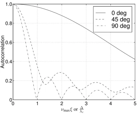
The form ofRE`(ξ)depends on angular location and spread of paths contributing to tap`(see Figures 4.3 and 4.4). We can expect that as the number of taps increases (due to increasing bandwidth), the angular spread corresponding to each tap decreases, since each tap “sees” fewer paths. This would mean that the coherence time (see Definition 3.9) of each tap, and hence the coherence time of the frequency selective channel, is a strong function of the bandwidthW.
1Typically, onlyE0(t)will have such a component due to a LOS path.
0 1 2 3 4 5 0 0.2 0.4 0.6 0.8 1.0 Autocorrelation
0 deg
45 deg
90 deg
PSfrag replacements νmaxξor λ∆cFigure 4.3: 0.5|RE`(ξ)|for various angular locations for spread of 60 deg.
0 2 4 6 8 10 0 0.2 0.4 0.6 0.8 1.0 Autocorrelation
0 deg
45 deg
90 deg
PSfrag replacements νmaxξor λ∆cFigure 4.4: 0.5|RE`(ξ)|for various angular locations for spread of 10 deg.
It is also of interest to compute the cross-correlation function ofE`(t)andEk(t), for`6=k, since the frequency
diversity afforded by the channel depends on cross-correlation between the taps. REkE`(ξ) =E[Ek(t+ξ)E ? `(t)] ≈X n β2nej2πνnξsinc[W (τ n−`/W)] sinc[W (τn−k/W)] = Z τds 0 Z νmax −νmax Ψ(ν, τ)ej2πνξsinc[W(τ−`/W)] sinc [W (τ−k/W)] dνdτ . (4.27)
From the above equation, one can see that the fading on neighboring taps can be correlated, except if the paths are clustered around the uniformly spaced tap centers.
If allow for flexibility in choosing the tap delays, instead of having them spaced uniformly in multiples of
1/W, we get the following approximation: h(t;τ)≈
LXc−1
`=0
E`(t)δ(τ−τ`) , (4.28)
whereLcis number of taps andτ`delay of tap`. If the tap delays are chosen to match cluster centers in delay
profile, then we get two beneficial outcomes. First, we may be able to approximate the channel with fewer taps, without wasting taps in portions of the delay profile that do not have significant received energy. Second, the taps will be more or less uncorrelated, i.e.,REkE`≈0, for`6=k.
4.3.2 JOINT DELAY-DOPPLER SAMPLED REPRESENTATION
In the previous section we developed a sampled delay representation for frequency-selective channels by ex-ploiting the fact that we observe the channel over a finite bandwidth W. We now combine this sampled representation with the one developed in Section 4.2 for frequency-flat fading to obtain a joint delay-Doppler sampled representation of the channel.
Each of the tapsE`(t)in the tapped delay line representation of (4.22) is bandlimited to a maximum frequency
of±νmax, just as the flat fading processE(t). As in Section 4.2, we assume that the channel is observed over
a finite time horizon [0, T], whereT < Tsmall. Then eachE`(t)has a sampled Doppler representation with 2M+ 1 =BdT samples of the form:
E`(t)≈ M X m=−M cm,` e j2πmt T , t∈[0, T]. (4.29) where cm,`= 1 T Z T 0 E`(t)e −j2πmt T dt =X n βnejϕne−jπmsinc[T(νn−m/T)] sinc[W(τn−`/W)] . (4.30)
Plugging approximation (4.29) into (4.22) yields the following approximate sampled representation forh(t;τ).
h(t;τ)≈ L X `=0 M X m=−M cm,` e j2πmt T δ(τ−`/W) , t∈[0, T]. (4.31) cV. V. Veeravalli, 2007 56
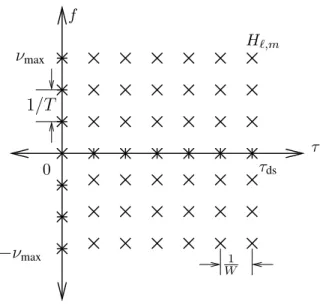
PSfrag replacements f τ −νmax νmax τds 0 1/T 1 W H`,m
Figure 4.5: Canonical joint delay-Doppler sampled representation.
Note that the coefficients cm,` in the above sampled representation represent uniform sampling in delay and
Doppler frequency. To further elucidate this point it is instructive to compare the sampled representation with the continuous delay-Doppler representation ofh(t;τ)in terms of the spreading functionC(ν, τ)(see (3.92)).
h(t;τ) = Z τds 0 Z νmax −νmax C(ν;τ)ej2πνtδ(t−τ)dν dτ (4.32) where C(ν, τ) =X n βnejϕn δ(ν−νn)δ(τ −τn). (4.33)
We now defineCb(ν, τ)as a smoothed version of the spreading function imposed by the finite signaling duration
and bandwidth,viz. b C(ν, τ) = Z τds 0 Z νmax −νmax C(ν0, τ0)e−jπT(ν−ν0)sinc(T(ν−ν0))sinc(W(τ −τ0))dν0dτ0. (4.34) Then it is clear from the above equation and (4.30) that
cm,`=Cb(m/T;`/W) . (4.35)
Thus the representation of (4.31) is essentially a sampled version of (4.32) commensurate with the sampling resolution afforded by the signal space: ∆τ = 1/W,∆ν = 1/T. Furthermore, the coefficients of the sampled representation are uniform samples of a smoothed version of the spreading function. The sampled delay-Doppler channel representation is illustrated in Figure 4.5).
4.3.3 STATISTICS OF THE SAMPLED REPRESENTATION
As we did previously in the case of sampled Doppler and sampled delay representations, we assume that the scattering is rich enough that the “sinc masks” corresponding to each coefficient in (4.30) capture a sufficiently
large number of paths2to apply the Central Limit Theorem. Under this assumption, if the paths contributing to cm,`do not include a specular component, thencm,`has Rayleigh first order statistics; otherwise, it has Ricean
statistics.
The correlation between the coefficients is easily shown to be
E[cm,`c?m0,`0] =e−jπ(m−m 0)Z τds 0 Z νmax −νmax Ψ(ν, τ)sinc[T(ν−m/T)] sincT(ν−m0/T)· sinc[W(τ−`/W)] sincW(τ −`0/W) dν dτ (4.36)
From the above expression, we note that for sufficiently smoothΨ(ν, ξ)(flat ideally), the correlation between different delay-Doppler coefficients is approximately zero as long as the indices are not too close to the end of their range. This follows from the orthogonality of the sinc basis functions.
The variation across blocks of durationTsmallis much more complicated since it is governed by the large scale variations. A special case of such variations in discussed below.
Block (Independent) Fading Channel Model
T
T
T Figure 4.6: Block Fading Model
Consider the situation where the channel is observed over blocks of duration T < Tsmall, but channel real-izations are independent from block to block. Such a scenario might arise in TDMA or frequency hopping systems, where consecutive blocks of the channel are well-separated in time or frequency. In this case the delay-Doppler coefficients remain constant over the each block, and change independently to new values from block to block. This model for fading is called theblock fading model.
A special case of the block fading model is one whereT is so small that T Bd < 1. This implies that one
Doppler tap is sufficient, i.e.,M = 0, and within each block
h(t;τ)≈ LX−1
`=0
c`δ(τ −`/W)=∆h(τ). (4.37)
This means that the channel is LTI within each block. This special case of the block fading model has been used extensively in information-theoretic capacity calculations for fading channels.
The block (independent) fading model can be generalized to allow for both time-selectivity within the block (T Bd > 1) as well as correlation across blocks. Such a model would be useful in scenarios where
indepen-dence cannot be justified using time or frequency hopping arguments. However, there could be spurious edge effects at the boundaries of blocks, and so one must be careful in developing such models.
2This assumption may not hold whenT and (or)W are large even if the scattering is rich. We discuss this in greater detail in
Section 4.4.