A New QoS-Aware Routing
Protocol for MANET Using
Artificial Neural Network
Prakash Srivastava and Rakesh Kumar
Department of Computer Science and Engineering, Madan Mohan Malaviya University of Technology, Gorakhpur, India
The explosive growth of Internet leads to increased diversity of applications. Multimedia applications, which are delay sensitive and include telephony, vi- deoconferencing etc. can benefit from this approach to satisfy their QoS routing requirement. Existing route discovery involves estimation of delay at every mobile node which involves calculation of queueing delay as well as contention delay. However, it is a complex procedure but it is required in fulfilling QoS routing requirements in MANET. Artificial neural networks are emerging as a promising technology which can be applied in networking field, simulating human mind in learning from experiences.We have utilized the ca-pability of artificial neural networks (ANN) for accu-rate prediction of end-to-end packet delay in MANET. Existing link failure strategy involves frequent route discoveries which incur high routing overhead and increased end-to-end delay. In this paper, efficient link failure recovery is also incorporated by utilizing multiple alternate paths in case of link failure, which is determined through signal intensity level and link expiration metric to provide link failure prediction be-fore it breaks up.The proposed methodology has been implemented in a computer simulation. Results show that our approach has been found outperforming to ex-isting approaches and has the potential to be applied in real world scenarios.
ACM CCS (2012) Classification: Networks → Net-work protocols → Network Layer Protocols → Rout-ing Protocols
Networks → Network types → Ad hoc networks → Mobile ad hoc networks
Keywords: MANET, QoS routing, neural networks, link failure
1. Introduction
Mobile ad hoc Network (MANET) is a self organized, infrastructureless wireless network without any centralized administration [1]. The
goal of QoS aware routing is to identify the op-timal path that satisfies the stringent require-ments of QoS parameters like delay, bandwidth, jitter etc. Multimedia applications such as audio and video have much more stringent QoS re-quirements. For a network to guarantee QoS de-liveries, it has to reserve and control resources like minimal bandwidth requirement and delay gaurantees. The main issues and challenges of MANET routing protocols are to deal with link failures and route recovery in these situations. The efficiency of route recovery affects the overall performance of MANETs. AODV has two route repair strategies to deal with link fail-ure. Routes are repaired by either reestablishing a new route starting from source node, or it can be locally repaired by the node that detects the link break along the end-to-end path [2]-[6]. The end-to-end delay in QoS routing consists of two types: contention delay and queueing de-lay. Contention delay consists of the latencies for data transmissions and retransmissions. On the other hand, queueing delay is the amount of time that the data packet waits until it gets the shared MAC layer interface. The estimation of end-to-end packet delay [7] in mobile ad hoc network environment is complex as it depends on significant variables such as path length from source to destination, average neighbours of intermediate hops, interference, medium ac-cess control protocol etc.
to the destination, it results in the decrease of the network throughput as well as in long de-lays. The problem gets worst when mobility is high. Our approach also focuses on estimation of link expiration metric (LET) and link fail-ure prediction [8] of next node link using sig-nal strength detection technique. If the sigsig-nal strength detection or LET is low, predecessor node searches an alternate route utilizing a mesh structure and establishes a path after re-ceiving acknowledgement from an alternate node to support effective link recovery strategy.
1.1. Contributions
Specific contribution of the paper focuses on designing a new QoS aware routing protocol for supporting delay sensitive applications. During route discovery process, end-to-end delay is pre-dicted using artificial neural network by taking into account parameters, viz.: average number of neighbours and hop length, which helps in identifying routes. An artificial neural network is a powerful tool [9] which has the property to learn, adapt and predict the principle of learn-ing from experiences. Besides this, efficient route recovery strategy is also incorporated by utilizing multiple alternate paths in case of link failure, which is determined through signal in-tensity level and link expiration metric to pro-vide link failure prediction before it breaks up. The proposed efficient route recovery strategy ensures lesser routing overhead, hence results in optimized network performance.
Furthermore, comprehensive performance eval-uation of the proposed approach with respect to varying scenarios of traffic load and mobility situations are analyzed. Comparison with exist-ing state of the art related scheme is also per-formed to validate performance improvement over existing one.
1.2. Challenges in QoS Routing
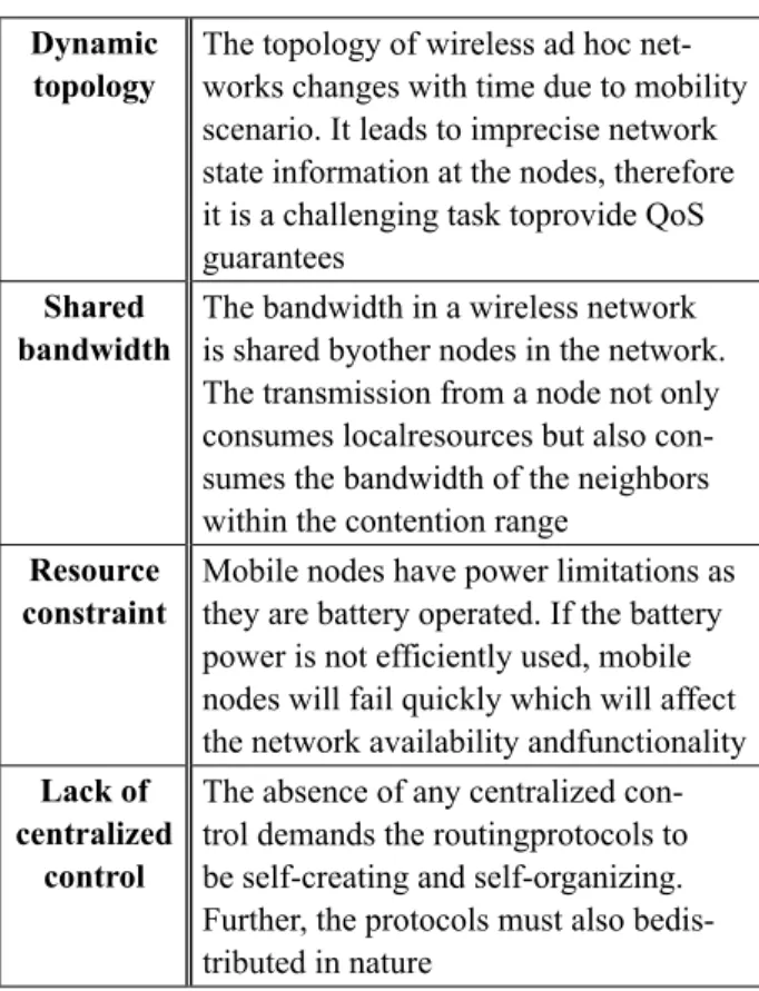
QoS routing has to consider application require-ments and the availability of network resources. Consequently, QoS routing in ad hoc networks exhibits great challenges which is reflected in Table 1.
Table 1. QoS routing challenges. Dynamic
topology The topology of wireless ad hoc net-works changes with time due to mobility scenario. It leads to imprecise network state information at the nodes, therefore it is a challenging task toprovide QoS guarantees
Shared
bandwidth The bandwidth in a wireless network is shared byother nodes in the network. The transmission from a node not only consumes localresources but also con-sumes the bandwidth of the neighbors within the contention range
Resource
constraint Mobile nodes have power limitations as they are battery operated. If the battery power is not efficiently used, mobile nodes will fail quickly which will affect the network availability andfunctionality Lack of
centralized control
The absence of any centralized con-trol demands the routingprotocols to be self-creating and self-organizing. Further, the protocols must also bedis-tributed in nature
The delay sensitive applications along with their maximum delay tolerance value are given in Table 2. If the value exceeds beyond this, the performance will degrade. Hence, the objective of QoS routing will not be fulfilled.
Table 2. Delay sensitive applications with their requirements.
Type of Applications One way delay tolerance value Voice over IP (VOIP) 150 ms
Video Conferencing 150 ms
IPTV 100 ms
Video on demand 50 ms
Gaming 50 ms
The rest of the paper is organized as follows: Section 2 describes related work about QoS routing and link failure recovery schemes. Sec-tion 3 presents our proposed QoS routing pro-tocol and neural network model. Section 4 re-marks the analytical validation of our proposed approach. Section 5 reflects our simulated and predicted results using Network training tool in MATLAB. Finally, in Section 6 we conclude the paper with directions of future work.
Lee et al. [15] proposed AODV-BR Backup
Routing, a modified protocol version of AODV which can be implemented in any demand uni-cast routing protocol to improve the reliable packet delivery in case of node movement and route breaks. The mess configuration provides multiple alternate routes and is constructed without extra overhead. This alternate route is utilized only when data packet cannot be de-livered through primary route. Therefore, pos-sibility of packet loss during handoff period can arise. This protocol also increased the number of route discovery processes because each time when a route fails, route discovery process is started by sending node. The performance of AODV-BR routing protocol decreases when the traffic load and mobility increase.
Gafur et al. [16] proposed an efficient local route repairing approach on the basis of TTL value as he considers that traditional route re-covery technique does not always provide op-timal path. In this paper they state that if there is any link breakage in the network, the alterna-tive route to the destination can be derived with a guarantee that it is not a suboptimal route. This paper does not concern the calculation of TTL value from the point of breakage in actual networking scenario.
3. Proposed QoS Routing Protocol
The proposed protocol focuses on QoS aware route discovery that provides the guaranteed end-to-end delay prediction and effective route recovery strategy throughout the communica-tion process. It will also focus on effective route maintenance strategy in case there is a link break or failure. The prediction of link failure is done before the actual failure occurs and alter-nate path is searched so that the data transmis-sion is continued without any further delay. The prediction of link failure is done on the basis of signal strength detection and link expiration time (LET) metric. The protocol predicts end-to-end delay dynamically on the basis of artificial neural network (ANN) for the QoS aware routing path to support the stringent re-quirements of delay sensitive applications. For route selection, it considers only those routes which have end-to-end delay, less than or equal
2. Related Work
Kuppusamy et al. [10] compared the perfor-mance of Temporary-Ordered Routing Algo-rithm (TORA) and routing on-demand acyclic multipath algorithms, but these algorithms re-quire additional control messages to construct and maintain alternate routes. TORA is a highly adaptive distributed routing algorithm which has been tailored for operation in a mobile net-working environment. The basic underlying routing mechanism of TORA is neither a dis-tance-vector nor a link-state algorithm, but it is one of a family of link-reversal algorithms. TORA routing protocol also degrades their per-formance because this protocol requires addi-tional control message for alternate route setup. Therefore, this protocol performs very poorly in high load and frequent disconnection envi-ronments.
Zafar et al. [11] proposed a new capacity-con-strained QoS-aware routing scheme referred to as the shortest multipath source: Q-SMS rout-ing which allows node to obtain and then use estimation of the residual capacity to make ap-propriate admission control decisions. In the Q-SMS scheme, there is no provisioning of any predictive way to anticipate a route break, which causes performance degradation, partic-ularly in mobile scenarios.
Singh et al. [12] proposed the prediction of end-to-end packet delay in Mobile Ad hoc Net-work using AODV, DSDV and DSR routing based on Generalized Regression Neural Net-work (GRNN) and Radial Basis function. How-ever, there is no provisioning of link recovery. Surjeet et al. [13] proposed a novel on demand QoS routing protocol MQAODV for band-width constrained delay sensitive applications in MANETs. It discovers routes based on band-width constrained path delay in addition to hop count. QoS is not guaranteed in case of route break or network partition, so this approach does not suit well for mobile topologies. The link failure prediction strategy is also not incor-porated in this scheme.
to the destination, it results in the decrease of the network throughput as well as in long de-lays. The problem gets worst when mobility is high. Our approach also focuses on estimation of link expiration metric (LET) and link fail-ure prediction [8] of next node link using sig-nal strength detection technique. If the sigsig-nal strength detection or LET is low, predecessor node searches an alternate route utilizing a mesh structure and establishes a path after re-ceiving acknowledgement from an alternate node to support effective link recovery strategy.
1.1. Contributions
Specific contribution of the paper focuses on designing a new QoS aware routing protocol for supporting delay sensitive applications. During route discovery process, end-to-end delay is pre-dicted using artificial neural network by taking into account parameters, viz.: average number of neighbours and hop length, which helps in identifying routes. An artificial neural network is a powerful tool [9] which has the property to learn, adapt and predict the principle of learn-ing from experiences. Besides this, efficient route recovery strategy is also incorporated by utilizing multiple alternate paths in case of link failure, which is determined through signal in-tensity level and link expiration metric to pro-vide link failure prediction before it breaks up. The proposed efficient route recovery strategy ensures lesser routing overhead, hence results in optimized network performance.
Furthermore, comprehensive performance eval-uation of the proposed approach with respect to varying scenarios of traffic load and mobility situations are analyzed. Comparison with exist-ing state of the art related scheme is also per-formed to validate performance improvement over existing one.
1.2. Challenges in QoS Routing
QoS routing has to consider application require-ments and the availability of network resources. Consequently, QoS routing in ad hoc networks exhibits great challenges which is reflected in Table 1.
Table 1. QoS routing challenges. Dynamic
topology The topology of wireless ad hoc net-works changes with time due to mobility scenario. It leads to imprecise network state information at the nodes, therefore it is a challenging task toprovide QoS guarantees
Shared
bandwidth The bandwidth in a wireless network is shared byother nodes in the network. The transmission from a node not only consumes localresources but also con-sumes the bandwidth of the neighbors within the contention range
Resource
constraint Mobile nodes have power limitations as they are battery operated. If the battery power is not efficiently used, mobile nodes will fail quickly which will affect the network availability andfunctionality Lack of
centralized control
The absence of any centralized con-trol demands the routingprotocols to be self-creating and self-organizing. Further, the protocols must also bedis-tributed in nature
The delay sensitive applications along with their maximum delay tolerance value are given in Table 2. If the value exceeds beyond this, the performance will degrade. Hence, the objective of QoS routing will not be fulfilled.
Table 2. Delay sensitive applications with their requirements.
Type of Applications One way delay tolerance value Voice over IP (VOIP) 150 ms
Video Conferencing 150 ms
IPTV 100 ms
Video on demand 50 ms
Gaming 50 ms
The rest of the paper is organized as follows: Section 2 describes related work about QoS routing and link failure recovery schemes. Sec-tion 3 presents our proposed QoS routing pro-tocol and neural network model. Section 4 re-marks the analytical validation of our proposed approach. Section 5 reflects our simulated and predicted results using Network training tool in MATLAB. Finally, in Section 6 we conclude the paper with directions of future work.
Lee et al. [15] proposed AODV-BR Backup
Routing, a modified protocol version of AODV which can be implemented in any demand uni-cast routing protocol to improve the reliable packet delivery in case of node movement and route breaks. The mess configuration provides multiple alternate routes and is constructed without extra overhead. This alternate route is utilized only when data packet cannot be de-livered through primary route. Therefore, pos-sibility of packet loss during handoff period can arise. This protocol also increased the number of route discovery processes because each time when a route fails, route discovery process is started by sending node. The performance of AODV-BR routing protocol decreases when the traffic load and mobility increase.
Gafur et al. [16] proposed an efficient local route repairing approach on the basis of TTL value as he considers that traditional route re-covery technique does not always provide op-timal path. In this paper they state that if there is any link breakage in the network, the alterna-tive route to the destination can be derived with a guarantee that it is not a suboptimal route. This paper does not concern the calculation of TTL value from the point of breakage in actual networking scenario.
3. Proposed QoS Routing Protocol
The proposed protocol focuses on QoS aware route discovery that provides the guaranteed end-to-end delay prediction and effective route recovery strategy throughout the communica-tion process. It will also focus on effective route maintenance strategy in case there is a link break or failure. The prediction of link failure is done before the actual failure occurs and alter-nate path is searched so that the data transmis-sion is continued without any further delay. The prediction of link failure is done on the basis of signal strength detection and link expiration time (LET) metric. The protocol predicts end-to-end delay dynamically on the basis of artificial neural network (ANN) for the QoS aware routing path to support the stringent re-quirements of delay sensitive applications. For route selection, it considers only those routes which have end-to-end delay, less than or equal
2. Related Work
Kuppusamy et al. [10] compared the perfor-mance of Temporary-Ordered Routing Algo-rithm (TORA) and routing on-demand acyclic multipath algorithms, but these algorithms re-quire additional control messages to construct and maintain alternate routes. TORA is a highly adaptive distributed routing algorithm which has been tailored for operation in a mobile net-working environment. The basic underlying routing mechanism of TORA is neither a dis-tance-vector nor a link-state algorithm, but it is one of a family of link-reversal algorithms. TORA routing protocol also degrades their per-formance because this protocol requires addi-tional control message for alternate route setup. Therefore, this protocol performs very poorly in high load and frequent disconnection envi-ronments.
Zafar et al. [11] proposed a new capacity-con-strained QoS-aware routing scheme referred to as the shortest multipath source: Q-SMS rout-ing which allows node to obtain and then use estimation of the residual capacity to make ap-propriate admission control decisions. In the Q-SMS scheme, there is no provisioning of any predictive way to anticipate a route break, which causes performance degradation, partic-ularly in mobile scenarios.
Singh et al. [12] proposed the prediction of end-to-end packet delay in Mobile Ad hoc Net-work using AODV, DSDV and DSR routing based on Generalized Regression Neural Net-work (GRNN) and Radial Basis function. How-ever, there is no provisioning of link recovery. Surjeet et al. [13] proposed a novel on demand QoS routing protocol MQAODV for band-width constrained delay sensitive applications in MANETs. It discovers routes based on band-width constrained path delay in addition to hop count. QoS is not guaranteed in case of route break or network partition, so this approach does not suit well for mobile topologies. The link failure prediction strategy is also not incor-porated in this scheme.
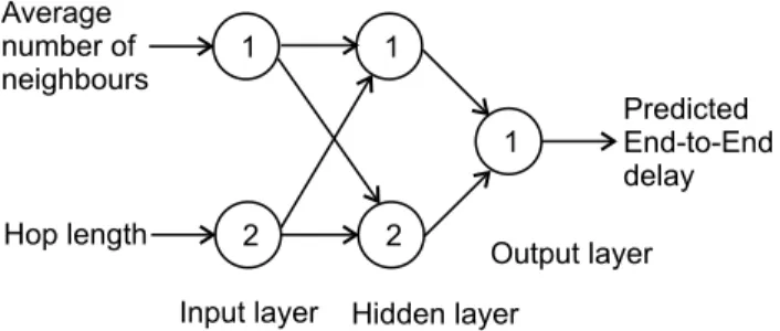
to that specified by the delay sensitive applica-tions. In this section, we describe our proposed protocol, which includes training of Multilayer perceptron on the basis of average number of neighbours (N) and hop length (H). These pa-rameters are chosen because they have a strong correlation and dependency on end-to-end de-lay. As average number of neighbours increases, there will be more collision and retransmission-leading to more delay. The increase in hop length results in accumulation of interface queuing delay. The predicted output is obtained as end-to-end delay. The accurate prediction given by neural network is used in QoS routing to identify optimal path that contains less end-to-end delay or, as per requirements, of de-lay sensitive applications. Hence, route discov-ery part is achieved with less routing overhead and complexity.
The Algorithm 1 for route discovery has been given below, along with neural network model which is depicted in Figure 1.
3.1. Neural Network Model
Our approach uses multilayer perceptron ar-chitecture of a neural network. The number of neurons in the input layer is enumerated as two as shown in Figure 1. The number of neurons
Algorithm 1. Route discovery. Step 1:
Step 2:
Step 3:
Step 4:
Step 5: Step 6:
if Source node S has no route to the destination then broadcast a RREQ
Training and testing data set for Neural Network is obtained on the basis of average number of neighbour nodes and hop length
For each routesi available {
predict end-to-end delayi on the basis of ANN }
if (end-to-end delayi < max_delay) then buffer the routei.
else try after some time when the mobility changes Identified routei will be used for QoS routing.
if destination node receives RERR packet due to local route repair fail
then pick up a fresh route, next better route, from buffer and unicasts RREP to the source
Figure 1. Multilayer Feed Forward Neural Network.
in the hidden layer has a tremendous influence on the final predicted output. Using less num-ber of neurons in the hidden layer will result in underfitting and too many neurons result in overfitting. Underfitting situation occurs when there are too few neurons in the hidden layers to adequately detect the signals in a compli-cated data set and overfitting situation occurs when the neural network has much information processing capacity that the limited amount of information contained in the training set is not enough to train all of the neurons in the hidden layers. Here, we choose to take two neurons in the hidden layer to avoid underfitting and over-fitting situations. The neural network is trained through Back propagation learning algorithm which itself comes under the category of su-pervised learning strategy. In the input layer we
used the linear transfer function as the activa-tion funcactiva-tion considering g=tanφ =1 and in the hidden and output layer we used sigmoidal function which behaves in a non linear activa-tion fashion which is shown below:
(
)
1
1 I
O
e−λ =
+ (3.1)
where,
λ → sigmoidal gain
O → Output at output layer
The sigmoidal gain λ provides a better method of coping with network paralysis and it can be applied to wide variety of applications so that faster training can be achieved.
3.2. Training Data Collection
The data sets used for training are obtained through simulated data using NS-2 tool. The random way point (RWP) movement pattern of mobile node is generated using BonnMotion [17] software. The maximum and minimum speed of a node is set to 10 m/s and 0.5 m/s re-spectively. The routing protocol used is Ad hoc on demand Distance Vector (AODV) routing. The IEEE 802.11 Distributed coordination function is used as MAC layer by every mobile node. The various scenarios of network are an-alyzed through simulation and their results are manipulated through trace file output using awk script. The end-to-end delay, average number of neighbors and hop length from source to desti-nation are obtained using trace files. The hun-dreds of data sets are obtained through various scenarios of hop length and average number of neighbors for training artificial neural network. Seventy data sets were used for training the
Figure 2. Searching and establishment of alternate path.
neural network, fifteen data sets were used for testing and remaining fifteen data sets were taken for validation.
3.3. Route Recovery Strategy
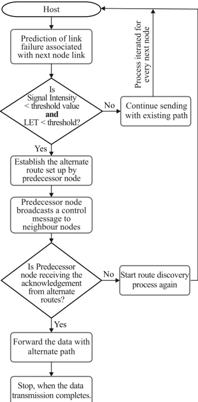
The link failure predicatibility is calculated on the basis of link expiration time (LET) and sig-nal strength detection. If the route is unstable or likely to be broken then alternate path is se-lected for transfer of control packets to identify whether the nodes in the alternate route have the routing entry to the destination. Whenever the receiving node detects a weak signal strength then it sends a control message to transmitting node, the node starts local route discovery pro-cess by broadcasting the control message with one hop count. The availability of alternate route is acknowledged by alternate nodes, lying in radio range of transmitting node. Acknowl-edgement message contains information (either P_ACK or N_ACK) and this route status is for-warded to the receiving node. The searching and establishment of alternate paths are depicted in Figure 2.
to that specified by the delay sensitive applica-tions. In this section, we describe our proposed protocol, which includes training of Multilayer perceptron on the basis of average number of neighbours (N) and hop length (H). These pa-rameters are chosen because they have a strong correlation and dependency on end-to-end de-lay. As average number of neighbours increases, there will be more collision and retransmission-leading to more delay. The increase in hop length results in accumulation of interface queuing delay. The predicted output is obtained as end-to-end delay. The accurate prediction given by neural network is used in QoS routing to identify optimal path that contains less end-to-end delay or, as per requirements, of de-lay sensitive applications. Hence, route discov-ery part is achieved with less routing overhead and complexity.
The Algorithm 1 for route discovery has been given below, along with neural network model which is depicted in Figure 1.
3.1. Neural Network Model
Our approach uses multilayer perceptron ar-chitecture of a neural network. The number of neurons in the input layer is enumerated as two as shown in Figure 1. The number of neurons
Algorithm 1. Route discovery. Step 1:
Step 2:
Step 3:
Step 4:
Step 5: Step 6:
if Source node S has no route to the destination then broadcast a RREQ
Training and testing data set for Neural Network is obtained on the basis of average number of neighbour nodes and hop length
For each routesi available {
predict end-to-end delayi on the basis of ANN }
if (end-to-end delayi < max_delay) then buffer the routei.
else try after some time when the mobility changes Identified routei will be used for QoS routing.
if destination node receives RERR packet due to local route repair fail
then pick up a fresh route, next better route, from buffer and unicasts RREP to the source
Figure 1. Multilayer Feed Forward Neural Network.
in the hidden layer has a tremendous influence on the final predicted output. Using less num-ber of neurons in the hidden layer will result in underfitting and too many neurons result in overfitting. Underfitting situation occurs when there are too few neurons in the hidden layers to adequately detect the signals in a compli-cated data set and overfitting situation occurs when the neural network has much information processing capacity that the limited amount of information contained in the training set is not enough to train all of the neurons in the hidden layers. Here, we choose to take two neurons in the hidden layer to avoid underfitting and over-fitting situations. The neural network is trained through Back propagation learning algorithm which itself comes under the category of su-pervised learning strategy. In the input layer we
used the linear transfer function as the activa-tion funcactiva-tion considering g=tanφ =1 and in the hidden and output layer we used sigmoidal function which behaves in a non linear activa-tion fashion which is shown below:
(
)
1
1 I
O
e−λ =
+ (3.1)
where,
λ → sigmoidal gain
O → Output at output layer
The sigmoidal gain λ provides a better method of coping with network paralysis and it can be applied to wide variety of applications so that faster training can be achieved.
3.2. Training Data Collection
The data sets used for training are obtained through simulated data using NS-2 tool. The random way point (RWP) movement pattern of mobile node is generated using BonnMotion [17] software. The maximum and minimum speed of a node is set to 10 m/s and 0.5 m/s re-spectively. The routing protocol used is Ad hoc on demand Distance Vector (AODV) routing. The IEEE 802.11 Distributed coordination function is used as MAC layer by every mobile node. The various scenarios of network are an-alyzed through simulation and their results are manipulated through trace file output using awk script. The end-to-end delay, average number of neighbors and hop length from source to desti-nation are obtained using trace files. The hun-dreds of data sets are obtained through various scenarios of hop length and average number of neighbors for training artificial neural network. Seventy data sets were used for training the
Figure 2. Searching and establishment of alternate path.
neural network, fifteen data sets were used for testing and remaining fifteen data sets were taken for validation.
3.3. Route Recovery Strategy
The link failure predicatibility is calculated on the basis of link expiration time (LET) and sig-nal strength detection. If the route is unstable or likely to be broken then alternate path is se-lected for transfer of control packets to identify whether the nodes in the alternate route have the routing entry to the destination. Whenever the receiving node detects a weak signal strength then it sends a control message to transmitting node, the node starts local route discovery pro-cess by broadcasting the control message with one hop count. The availability of alternate route is acknowledged by alternate nodes, lying in radio range of transmitting node. Acknowl-edgement message contains information (either P_ACK or N_ACK) and this route status is for-warded to the receiving node. The searching and establishment of alternate paths are depicted in Figure 2.
Prediction of link failure associated with next node link
No
Yes
No
Yes
Host
Is Signal Intensity < threshold value
LET < threshold?
and
Establish the alternate route set up by predecessor node
Predecessor node broadcasts a control
message to neighbour nodes
Is Predecessor
node receiv the
acknowledgement from alternate
routes? ing
Forward the data with alternate path
Stop, when the data transmission completes.
Continue sending with existing path
Process iterated for every next node
Start route discovery process again
Figure 3. Flow chart for route maintainenance.
3.3.1. Signal Strength Detection
The strength of a packet signal, which a node receives is obtained as per the following equa-tion [18]. The threshold value considered here is 40 dBµ (dB-microvolts per meter).
2 2 4
t r t r t
r p G G H H
p
d =
(3.2) where pr← strength of received signal
pt←strength of transmitted signal
Gr← antenna gain of receiver
Gt←antenna gain of transmitter,
Hr← antenna altitude of receiver
Ht← antenna altitude of transmitter
d ← distance between sending and receiving node is given as per equation 3.3:
2 2
4 t r t r t
r p G G H H d
p =
(3.3)
3.3.2 Link Expiration Time (LET)
Let i and j be two neighbouring wireless nodes in a route with (xi, yi) and (xj, yj) coordinates
respectively. Also, let vi and vj represent the
ve-locity of the node i and node j moving in the direction of θi and θj respectively. For the
trans-mission range r of node i (as shown in Figure 4) for link i to j to be active, d must be less than
r; if the value of d increases, the route break-age may occur and the link becomes unstable. Consequently, determination of path stability is relevant before data transmission achieves the desired level of quality of service. The link ex-piration time [19] is calculated with the help of equation 3.4:
2 2 2 2 2 2
(ab cd) (a c r) (ad bc)
LET
a c
− + + + − −
=
+ (3.4)
where
a = vi cosθi – vj cosθj, b = xi – xj, c = vi sinθi
– vj sinθj and d = yi – yj.
d
Node transmisson range
j
Node transmisson range
i j
i
Figure 4. Link expiration range.
4. Analytical Model
The analytical model is based on IEEE 802.11 protocol for Wireless Local Area Networks (WLAN) and most Wireless LAN and MANETs use this standard. This standard operates in two modes: DCF (Distributed Coordination Func-tion) and PCF (Point Coordination FuncFunc-tion). A mobile node M transmits in DCF mode using
RTS and CTS handshakes to avoid hidden ter-minal problem. The delay [20] at each node is calculated with the help of following equations:
_
( ) ( _ ( ))
(1 ( )) ( + ( ))+( / )
i idle
i idle
forwarding delay
P DIFS DIFS avg bt DA i
P DIFS SIFS DB i L R
=
× + +
+ − ×
(4.1)
where i ( )
idle
P t is the probability that mobile
nodei detects no other mobile node
transmit-ting data during time interval 't' and is given by i ( ) t
idle
P t =e−λ, λ is the aggregate arrival rate
including neighbour node at mobile node MNi.
DA(i) is expected delay encountered in the at-tempt state and is given by:
( ) ( ) ( 2 )
(1 ( )) ( +2 + ( ))
i idle
i idle
DA i P slot RTS SIFS CTS
P slot RTS SIFS DB i
= × + × +
+ − × ×
(4.2)
DB(i) is expected delay encountered during back-off state and is given by:
( ) [1/{ ( ) ( )}]
[ ( ) ( _
+ +2 + ( ) )]
+[1 ( ) ]
i i
idle idle
i idle
i idle i
idle
DB i P DIFS P slot
P DIFS DIFS avg bt
RTS SIFS P slot CTS
P DIFS X
= ×
× × +
× ×
− ×
(4.3)
avg _bt is a random back-off time interval be-fore transmission and is given by:
4
1 0
5 4
_
[ ( ) (1 ( )) 2 ]
+(1 ( )) 2
i i n n
idle idle
n
i idle avg bt
P slot P slot W
P slot W
− =
=
× − × ×
− × ×
∑
(4.4) Algorithm 2. Route maintenance.
Step 1: Step 2:
Step 3: Step 4: Step 5:
Step 6:
Step 7: Step 8: Step 9: Step 10:
Step 11: Step 12:
Calculate signal strength by each mobile and stationary node as per equation 3.2 if (computed signal strength <= threshold value) and (LET<=1)
then
Receiving node sends a message to the predecessor node. else go to step 12
Predecessor node broadcasts control message to its neighbors if Predecessor node receives acknowledgement from its neighbors then
if reply message includes P_ACK
then Alt-Route: = P_ACK //P_ACK shows availability of alternate route else if Alt-Route: = N_ACK //N_ACK shows unavailability of alternate route else Alt-Route: = NULL
Predecessor node forwards Alt-Route status to receiving node. if linkfailureoccurs
then
if Alt-Route = = P-ACK then
go to Step 12
Send RERR message to source
3
X RTS= + ×SIFS CTS L ACK+ + + (4.5)
L and R are packet length and data rate respec-tively. W is contention window size whereas
ACK is length of acknowledgement packet. In wireless links, the propagation delays are very small and almost equal for each hop along the path. So, here we assume that the propagation delay is negligible.
4.1. Network Model
We assume that the network consists of N
nodes that are distributed uniformly and inde-pendently over a rectangular area. Each node in the network can act as a source, destination and/or relay of packets. The radio transmission range of each node is assumed to have an equal transmission range, denoted by d. Let dij denote
the distance between node i and j. Nodes i and
j are said to be neighbours if they can directly communicate with each other i.e., if dij ≤ d.
The transmission rate is R bits/seconds. In our model, we assume that average packet arrival rate at a mobile node is λ packets/sec, which includes packets generated by the mobile node itself as well as packets arrived from neighbour nodes given by the following equation:
λ= ×n λM (4.6) where λM is the number of packets generated by
mobile node M itself and n consists of neigh-boring nodes including itself. Further, the size of each packet is assumed to be constant.
4.2. Average Hop Count
The average hop count is defined as the number of hops between an arbitrary source and desti-nation in the network. The average number of hops traversed per packet navg in an ad hoc
net-work is given by the following equation: navg E S{ }
d
= (4.7)
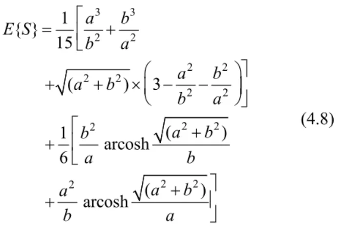
where E{S} is expected distance between two nodes in a rectangular area and is given by [21] as follows:
3 3 2 2
2 2 2 2
2 2 2 2 2
2 2 2
1 { }
15
( ) 3
( )
1 arcosh 6
( )
arcosh
a b
E S
b a
a b
a b
b a
a b
b
a b
a b
a
b a
= +
+ + × − −
+
+
+
+
(4.8)
where a and b denote its length and breadth re-spectively (in meters) for a terrain of network size
a × b. Here arcosh(x) is substituted in place of ln
(
x+ (x2−1))
.4.3. End-to-End Delay Analysis
In mobile ad hoc network, end-to-end delay is the delay encountered by a packet, which is evaluated from the time the packet is generated to the time the source node receives an ACK indicating successful reception of the packet by the destination node. The end-to-end packet delay consists of MAC delay and transmission delay experienced at the source node as well as intermediate nodes. If Dhop is one hop delay and
average number of hops traversed per packet between a source and a destination is given by navg, then the average end-to-end delay per
packet i.e. DEtoE can be obtained by the
follow-ing equation:
DEtoE = navg×Dhop (4.9)
where navg is obtained from equation 4.7.
4.4. Proposed Approach Analytical Validation
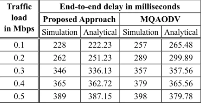
The comparison is done between the transmis-sion delay obtained by analytical model with the results obtained by simulation analysis. The simulation parameters used are as given in Ta-ble 4. TaTa-ble 3 shows average end-to-end delay per packet for different traffic load conditions obtained analytically using equation 4.9, and through simulation of our protocol. It is
ob-served that there is only a slight deviation of results obtained through simulation and analyt-ical approach.
Table 3. Analytical vs simulation results of end-to-end delay.
Traffic load in Mbps
End-to-end delay in milliseconds Proposed Approach MQAODV Simulation Analytical Simulation Analytical 0.1 228 222.23 257 265.48 0.2 262 251.23 289 299.89 0.3 346 336.13 357 357.56 0.4 365 362.72 379 365.56 0.5 389 387.15 398 379.78
5. Simulation Results and Discussion
The performance of our proposed approach is simulated using NS-2 simulator, for simulation purpose we have used the parameters given in Table 4. The network scenario consists of fixed number of nodes which is 50 in this case. The network topology consists of 1200 m × 800 m rectangular area. Nodes are generating con-stant bit rate (CBR) traffic with a packet of 512 bytes. The distributed coordination func-tion IEEE 802.11 is used in MAC layer. The interface queue size is considered to be 50. The mobility model used was Random waypoint. All simulations were run for the duration of 700 seconds.Table 4. Simulation parameters. Parameters Values Number of mobile nodes 50
Number of corresponding hosts 6
Topology size 1200X800 m
Traffic type CBR
Packet size 512 bytes Wireless transmission range 250 m
Packet sending rate 5 packets/second Mobility model Random waypoint Length of interface queue 50 packets Link level layer IEEE 802.11 DCF Speed of a mobile node 10 m/s
Simulation time 700 seconds
5.1. Movement Model
The wireless channel used is based on two ray ground radio propagation model. The mobility model used in simulation is the Random Way-point Model. Mobility model is generated using setdest utility. Setdest generates random posi-tions of nodes in the network with specified mobility and pause time. The command used is: /setdest –n 〈num of nodes〉 –p 〈pause time〉 –M 〈max speed〉 –t 〈simu time〉 –x 〈max x〉 –y 〈max y〉> 〈trace filename〉
5.2. Traffic Model
All data packets are CBR (constant bit rate) and the size of each packet is 512 bytes. A packet-transmission rate of 20 Kbps is considered in this scenario. The connection pattern is gen-erated using cbrgen. The command used is: ns cbrgen.tcl [–type cbr|tcp] [–nn nodes] [–seed seed] [–mc connections] [–rate rate]
5.3. Performance Metrics
The following performance metrics have been used to evaluate the performance of the pro-posed protocol
● Packet Delivery Ratio (pdr): It is the ratio between the received packets at the desti-nation and number of packets generated by the sources.
total number of received packets
total number of sent packets by the source 100
pdr= ×
● Routing Overhead: It is defined as the
to-tal number of control messages, including route discovery, sent out during the sce-nario.
1
n
overhead i
i
R Overhead
=
=
∑
,where n is the number of nodes.
● End-to-End Delay: The time taken by the
3
X RTS= + ×SIFS CTS L ACK+ + + (4.5)
L and R are packet length and data rate respec-tively. W is contention window size whereas
ACK is length of acknowledgement packet. In wireless links, the propagation delays are very small and almost equal for each hop along the path. So, here we assume that the propagation delay is negligible.
4.1. Network Model
We assume that the network consists of N
nodes that are distributed uniformly and inde-pendently over a rectangular area. Each node in the network can act as a source, destination and/or relay of packets. The radio transmission range of each node is assumed to have an equal transmission range, denoted by d. Let dij denote
the distance between node i and j. Nodes i and
j are said to be neighbours if they can directly communicate with each other i.e., if dij ≤ d.
The transmission rate is R bits/seconds. In our model, we assume that average packet arrival rate at a mobile node is λ packets/sec, which includes packets generated by the mobile node itself as well as packets arrived from neighbour nodes given by the following equation:
λ= ×n λM (4.6) where λM is the number of packets generated by
mobile node M itself and n consists of neigh-boring nodes including itself. Further, the size of each packet is assumed to be constant.
4.2. Average Hop Count
The average hop count is defined as the number of hops between an arbitrary source and desti-nation in the network. The average number of hops traversed per packet navg in an ad hoc
net-work is given by the following equation: navg E S{ }
d
= (4.7)
where E{S} is expected distance between two nodes in a rectangular area and is given by [21] as follows:
3 3 2 2
2 2 2 2
2 2 2 2 2
2 2 2
1 { }
15
( ) 3
( )
1 arcosh 6
( )
arcosh
a b
E S
b a
a b
a b
b a
a b
b
a b
a b
a
b a
= +
+ + × − −
+
+
+
+
(4.8)
where a and b denote its length and breadth re-spectively (in meters) for a terrain of network size
a × b. Here arcosh(x) is substituted in place of ln
(
x+ (x2−1))
.4.3. End-to-End Delay Analysis
In mobile ad hoc network, end-to-end delay is the delay encountered by a packet, which is evaluated from the time the packet is generated to the time the source node receives an ACK indicating successful reception of the packet by the destination node. The end-to-end packet delay consists of MAC delay and transmission delay experienced at the source node as well as intermediate nodes. If Dhop is one hop delay and
average number of hops traversed per packet between a source and a destination is given by navg, then the average end-to-end delay per
packet i.e. DEtoE can be obtained by the
follow-ing equation:
DEtoE = navg×Dhop (4.9)
where navg is obtained from equation 4.7.
4.4. Proposed Approach Analytical Validation
The comparison is done between the transmis-sion delay obtained by analytical model with the results obtained by simulation analysis. The simulation parameters used are as given in Ta-ble 4. TaTa-ble 3 shows average end-to-end delay per packet for different traffic load conditions obtained analytically using equation 4.9, and through simulation of our protocol. It is
ob-served that there is only a slight deviation of results obtained through simulation and analyt-ical approach.
Table 3. Analytical vs simulation results of end-to-end delay.
Traffic load in Mbps
End-to-end delay in milliseconds Proposed Approach MQAODV Simulation Analytical Simulation Analytical 0.1 228 222.23 257 265.48 0.2 262 251.23 289 299.89 0.3 346 336.13 357 357.56 0.4 365 362.72 379 365.56 0.5 389 387.15 398 379.78
5. Simulation Results and Discussion
The performance of our proposed approach is simulated using NS-2 simulator, for simulation purpose we have used the parameters given in Table 4. The network scenario consists of fixed number of nodes which is 50 in this case. The network topology consists of 1200 m × 800 m rectangular area. Nodes are generating con-stant bit rate (CBR) traffic with a packet of 512 bytes. The distributed coordination func-tion IEEE 802.11 is used in MAC layer. The interface queue size is considered to be 50. The mobility model used was Random waypoint. All simulations were run for the duration of 700 seconds.Table 4. Simulation parameters. Parameters Values Number of mobile nodes 50
Number of corresponding hosts 6
Topology size 1200X800 m
Traffic type CBR
Packet size 512 bytes Wireless transmission range 250 m
Packet sending rate 5 packets/second Mobility model Random waypoint Length of interface queue 50 packets Link level layer IEEE 802.11 DCF Speed of a mobile node 10 m/s
Simulation time 700 seconds
5.1. Movement Model
The wireless channel used is based on two ray ground radio propagation model. The mobility model used in simulation is the Random Way-point Model. Mobility model is generated using setdest utility. Setdest generates random posi-tions of nodes in the network with specified mobility and pause time. The command used is: /setdest –n 〈num of nodes〉 –p 〈pause time〉 –M 〈max speed〉 –t 〈simu time〉 –x 〈max x〉 –y 〈max y〉> 〈trace filename〉
5.2. Traffic Model
All data packets are CBR (constant bit rate) and the size of each packet is 512 bytes. A packet-transmission rate of 20 Kbps is considered in this scenario. The connection pattern is gen-erated using cbrgen. The command used is: ns cbrgen.tcl [–type cbr|tcp] [–nn nodes] [–seed seed] [–mc connections] [–rate rate]
5.3. Performance Metrics
The following performance metrics have been used to evaluate the performance of the pro-posed protocol
● Packet Delivery Ratio (pdr): It is the ratio between the received packets at the desti-nation and number of packets generated by the sources.
total number of received packets
total number of sent packets by the source 100
pdr= ×
● Routing Overhead: It is defined as the
to-tal number of control messages, including route discovery, sent out during the sce-nario.
1
n
overhead i
i
R Overhead
=
=
∑
,where n is the number of nodes.
● End-to-End Delay: The time taken by the
5.4. Performance Evaluation of Delay Prediction using MATLAB
The neural network is realized using MATLAB software, back propagation training algorithm and random data division technique. The per-formance metric discussed in the following is used as a goodness measure to verify the cor-rectness of neural network architecture used for our predicted results.
The correlation coefficient (rc) given in
equa-tion 5.1 indicates how the predicted values vary from the target values. Oi represents the
ob-served values for ithperiod during simulation taking the varying scenario as discussed in sub-section 3.2. Om represents the mean of the
ob-served values during simulation. Pi and Pm
indi-cate the predicted delay for ith period and mean of the predicted delay respectively obtained from the neural network. Table 4 reflects the goodness measure of accuracy of results ob-tained by proposed neural network model.
1
2 2
1 1
( )( )
( ) ( )
n
i m i m
i
c n n
i m i m
i i
O O P P r
O O P P
=
= =
− −
=
− −
∑
∑
∑
(5.1)The root mean squared error (rmse) in equa-tion 5.2 reflects the deviaequa-tion between the
ac-Figure 5. Mean squared error.
tual value observed from the simulation and predicted values obtained from neural network architecture. The significant feature of rmse is to uncover large errors rather than small errors. 2
1
1
rmse n ( i i)
i
O P
n =
=
∑
− (5.2)The mean absolute error in equation 5.3 indi-cates the absolute difference between the pre-dicted and observed value. The error is con-sidered in terms of absolute value of the error terms.
1
1
mae n i i
i
O P
n =
=
∑
− (5.3)The graph illustrating the mean squared error, see Figure 5, decreases as the number of itera-tions increases. When neural network is trained after several iterations it produces accurate de-lay prediction.
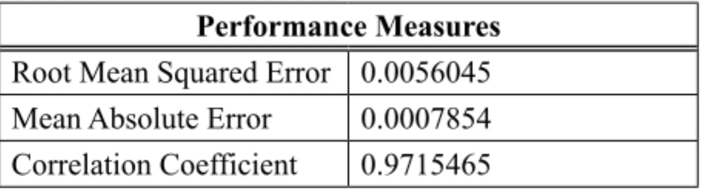
The error histogram shown in Figure 6 illustrates the stages of training, validation and testing along with the deviation between actual and tar-get outputs. Once the artificial neural network is trained, the errors will be minimized. Accuracy of prediction is shown in Table 5, with the re-sults obtained using 100 sets of data from NS-2 trace by varying simulation scenarios. Seventy
Figure 6. Error histogram reflecting deviation between targets and outputs. sets of data are used for training multilayer feed
forward neural network and remaining thirty sets of data are used for testing and validation.
Table 5. Goodness measure. Performance Measures Root Mean Squared Error 0.0056045 Mean Absolute Error 0.0007854 Correlation Coefficient 0.9715465
The graph shown in Figure 7 illustrates the de-lay prediction obtained using neural network tool and actual delay realized through
simula-0.7
0.6
0.5
0.4
0.3
0.2
0.1
0
End-to-End delay
Time
0 5 10 15 20 25 30 35
Actual Predicted
Figure 7. Actual vs predicted end-to-end delay.
tions. The predicted results do not show much deviation, hence our proposed neural network architecture is effectively trained and produces correct results. The comparison results are shown here to ensure that end-to-end delay pre-dicted through multilayer feed forward neural network is similar to end-to-end delay results obtained through computer simulation. The predicted end-to-end delay using multilayer feed forward neural network architecture is used in QoS aware route discovery phase.
5.4.1. Effect of Node Mobility
A simulation model consisting of 50 mobile nodes with 6 active sessions, each with 5 pack-ets/second arrival rate and variable pause time was considered for simulation. To study the ef-fect of mobility, pause time was varied from 0 to 700 seconds with steps of 100 seconds.
exist-5.4. Performance Evaluation of Delay Prediction using MATLAB
The neural network is realized using MATLAB software, back propagation training algorithm and random data division technique. The per-formance metric discussed in the following is used as a goodness measure to verify the cor-rectness of neural network architecture used for our predicted results.
The correlation coefficient (rc) given in
equa-tion 5.1 indicates how the predicted values vary from the target values. Oi represents the
ob-served values for ithperiod during simulation taking the varying scenario as discussed in sub-section 3.2. Om represents the mean of the
ob-served values during simulation. Pi and Pm
indi-cate the predicted delay for ith period and mean of the predicted delay respectively obtained from the neural network. Table 4 reflects the goodness measure of accuracy of results ob-tained by proposed neural network model.
1
2 2
1 1
( )( )
( ) ( )
n
i m i m
i
c n n
i m i m
i i
O O P P r
O O P P
=
= =
− −
=
− −
∑
∑
∑
(5.1)The root mean squared error (rmse) in equa-tion 5.2 reflects the deviaequa-tion between the
ac-Figure 5. Mean squared error.
tual value observed from the simulation and predicted values obtained from neural network architecture. The significant feature of rmse is to uncover large errors rather than small errors. 2
1
1
rmse n ( i i)
i
O P
n =
=
∑
− (5.2)The mean absolute error in equation 5.3 indi-cates the absolute difference between the pre-dicted and observed value. The error is con-sidered in terms of absolute value of the error terms.
1
1
mae n i i
i
O P
n =
=
∑
− (5.3)The graph illustrating the mean squared error, see Figure 5, decreases as the number of itera-tions increases. When neural network is trained after several iterations it produces accurate de-lay prediction.
The error histogram shown in Figure 6 illustrates the stages of training, validation and testing along with the deviation between actual and tar-get outputs. Once the artificial neural network is trained, the errors will be minimized. Accuracy of prediction is shown in Table 5, with the re-sults obtained using 100 sets of data from NS-2 trace by varying simulation scenarios. Seventy
Figure 6. Error histogram reflecting deviation between targets and outputs. sets of data are used for training multilayer feed
forward neural network and remaining thirty sets of data are used for testing and validation.
Table 5. Goodness measure. Performance Measures Root Mean Squared Error 0.0056045 Mean Absolute Error 0.0007854 Correlation Coefficient 0.9715465
The graph shown in Figure 7 illustrates the de-lay prediction obtained using neural network tool and actual delay realized through
simula-0.7
0.6
0.5
0.4
0.3
0.2
0.1
0
End-to-End delay
Time
0 5 10 15 20 25 30 35
Actual Predicted
Figure 7. Actual vs predicted end-to-end delay.
tions. The predicted results do not show much deviation, hence our proposed neural network architecture is effectively trained and produces correct results. The comparison results are shown here to ensure that end-to-end delay pre-dicted through multilayer feed forward neural network is similar to end-to-end delay results obtained through computer simulation. The predicted end-to-end delay using multilayer feed forward neural network architecture is used in QoS aware route discovery phase.
5.4.1. Effect of Node Mobility
A simulation model consisting of 50 mobile nodes with 6 active sessions, each with 5 pack-ets/second arrival rate and variable pause time was considered for simulation. To study the ef-fect of mobility, pause time was varied from 0 to 700 seconds with steps of 100 seconds.
exist-ing approaches. The average end-to-end delay with variable pause time is depicted in Figure 8.
Figure 8. End-to-end delay vs pause time.
Routing Overhead. Routing overhead in our proposed approach is smaller than MQAODV, as the route maintenance procedure discussed in Algorithm 2 does not involve subsequent route error messages in case of link failure. Therefore the number of messages generated will be less. The routing overhead, with varying pause time of the mobile nodes, is depicted in Figure 9.
Figure 9. Routing overhead vs pause time.
Packet Delivery Ratio. With high mobility, the proposed approach reflects less packet delivery ratio as compared to MQAODV in the case of
low pause time. With high mobility, interfer-ence from neighbouring nodes becomes high, and more collision and retransmission occur. As mobility decreases, pause time becomes greater than 300 seconds, and the proposed approach outperforms MQAODV because of its better route maintenance policy. At low mobility, few link breaks occur and the routes are balanced. The packet delivery ratio with variable pause time of the mobile nodes is shown in Figure 10.
Figure 10. Packet delivery ratio vs pause time.
5.4.2 Effect of Traffic Load
In our model, different traffic loads were simu-lated varying from 0.1 to 0.6 Mbps. A simula-tion model consisting of 50 mobile nodes using random waypoint mobility model with 400 sec pause time and 5 packets/sec arrival rate were considered for simulation. This section dis-cusses the comparative evaluation of our pro-posed approach and MQAODV.
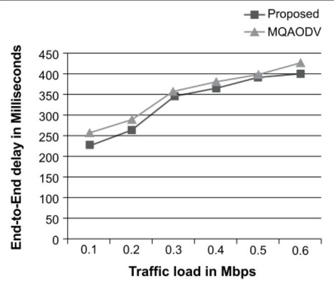
End-to-End Delay. The end-to-end delay of our proposed approach is lesser than MQAODV in the situation of low and high traffic. The pre-dicted end-to-end delay used in our scheme for identifying path having low delay latency. Furthermore, as the traffic load increases, inter-ference with neighbour nodes increases, result-ing in frequent route changes. Consequently, contention delay will be higher. However, our proposed approach performs better even in high traffic situations, since multilayer feed forward
neural network architecture is trained with varying scenarios. The end-to-end delay with varying traffic load is shown in Figure 11.
Figure 11. End-to-end delay vs traffic load.
Routing Overhead. The routing overhead in our proposed approach is lesser than MQAODV as it uses efficient link failure strategy to pre-serve the QoS requirements. At high traffic, as the load on the system is greater, the nodes be-come congested, which consequently increases the routing overhead. The routing overhead with varying traffic load is shown in Figure 12.
Figure 12. Routing overhead vs traffic load.
Packet Delivery Ratio. Figure 13 reflects the performance in our approach in terms of packet delivery ratio, the performance is shown better
than MQAODV at high traffic.This approach has an efficient route recovery strategy so it re-sults in less frequent route failure hence lesser packet drops, therefore enhanced throughput is achieved.
Figure 13. Packet delivery ratio vs traffic load.
6. Conclusion
ing approaches. The average end-to-end delay with variable pause time is depicted in Figure 8.
Figure 8. End-to-end delay vs pause time.
Routing Overhead. Routing overhead in our proposed approach is smaller than MQAODV, as the route maintenance procedure discussed in Algorithm 2 does not involve subsequent route error messages in case of link failure. Therefore the number of messages generated will be less. The routing overhead, with varying pause time of the mobile nodes, is depicted in Figure 9.
Figure 9. Routing overhead vs pause time.
Packet Delivery Ratio. With high mobility, the proposed approach reflects less packet delivery ratio as compared to MQAODV in the case of
low pause time. With high mobility, interfer-ence from neighbouring nodes becomes high, and more collision and retransmission occur. As mobility decreases, pause time becomes greater than 300 seconds, and the proposed approach outperforms MQAODV because of its better route maintenance policy. At low mobility, few link breaks occur and the routes are balanced. The packet delivery ratio with variable pause time of the mobile nodes is shown in Figure 10.
Figure 10. Packet delivery ratio vs pause time.
5.4.2 Effect of Traffic Load
In our model, different traffic loads were simu-lated varying from 0.1 to 0.6 Mbps. A simula-tion model consisting of 50 mobile nodes using random waypoint mobility model with 400 sec pause time and 5 packets/sec arrival rate were considered for simulation. This section dis-cusses the comparative evaluation of our pro-posed approach and MQAODV.
End-to-End Delay. The end-to-end delay of our proposed approach is lesser than MQAODV in the situation of low and high traffic. The pre-dicted end-to-end delay used in our scheme for identifying path having low delay latency. Furthermore, as the traffic load increases, inter-ference with neighbour nodes increases, result-ing in frequent route changes. Consequently, contention delay will be higher. However, our proposed approach performs better even in high traffic situations, since multilayer feed forward
neural network architecture is trained with varying scenarios. The end-to-end delay with varying traffic load is shown in Figure 11.
Figure 11. End-to-end delay vs traffic load.
Routing Overhead. The routing overhead in our proposed approach is lesser than MQAODV as it uses efficient link failure strategy to pre-serve the QoS requirements. At high traffic, as the load on the system is greater, the nodes be-come congested, which consequently increases the routing overhead. The routing overhead with varying traffic load is shown in Figure 12.
Figure 12. Routing overhead vs traffic load.
Packet Delivery Ratio. Figure 13 reflects the performance in our approach in terms of packet delivery ratio, the performance is shown better
than MQAODV at high traffic.This approach has an efficient route recovery strategy so it re-sults in less frequent route failure hence lesser packet drops, therefore enhanced throughput is achieved.
Figure 13. Packet delivery ratio vs traffic load.