Navigating Dynamic Environments
with Trajectory Deformation
Thierry Fraichard and Vivien Delsart
INRIA, LIG-CNRS and Grenoble University, FrancePath deformation is a technique that was introduced to generate robot motion wherein a nominal path, that had been computed beforehand, was continuously deformed on-line in response to unforeseen obstacles. In an effort to improve path deformation, this paper presents a trajectory deformation scheme. The main idea is that by incorporating the time dimension and hence information on the obstacles’ future behaviour, quite a number of situ-ations where path deformation would fail can be handled. The trajectory represented as a discrete space-time curve is subject to deformation forces both external(to avoid collision with the obstacles) and internal(to maintain trajectory feasibility and connectivity). The trajectory deformation scheme has been tested successfully on a planar robot with double integrator dynamics moving in dynamic environments.
Keywords: mobile robots, autonomous navigation, colli-sion avoidance, motion deformation
1. Introduction
Where to move next? is a key question for an autonomous robotic system. This fundamen-tal issue has been largely addressed in the past forty years. Many motion determination strate-gies have been proposed(see Lavalle(2006)for a review). They can broadly be classified into
deliberative versus reactive strategies: delib-erative strategies aim at computing a complete motion all the way to the goal, whereas reac-tive strategies determine the motion to execute during the next few time-steps only. Delibera-tive strategies have to solve a motion planning problem. They require a model of the environ-ment as complete as possible and their intrinsic complexity is such that it may preclude their application in dynamic environments. Reactive strategies, on the other hand, can operate on-line using local sensor information: they can be
used in any kind of environment whether un-known, changing or dynamic, but convergence towards the goal is difficult to guarantee. To bridge the gap between deliberative and reac-tive approaches, a complementary approach has been proposed based uponmotion deformation. The principle is simple: a complete motion to the goal is computed first using a priori informa-tion. It is then passed on to the robotic system for execution. During the course of the execu-tion, the still-to-be-executed part of the motion is continuously deformed in response to sensor information acquired on-line, thus accounting for the incompleteness and inaccuracies of the a priori world model. Deformation usually re-sults from the application of constraints, both external(imposed by the obstacles)and internal
(to maintain motion feasibility and connectiv-ity). Provided that the motion connectivity can be maintained, convergence towards the goal is achieved.
The different motion deformation techniques that have been proposed Quinlan and Khatib
(1993); Khatib et al. (1997); Brock and Khatib
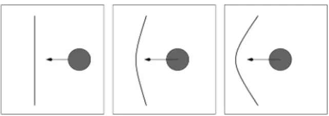
(by slowing down or accelerating). To achieve this, it is necessary to depart from the path de-formation paradigm and resort totrajectory de-formationinstead. A trajectory is essentially a geometric path parametrized by time. It tells us where the robotic system should be, but also when and with what velocity. Unlike path defor-mation wherein spatial defordefor-mation only takes place, trajectory deformation features both spa-tial and temporal deformations meaning that the planned velocity of the robotic system can be altered thus permitting to handle gracefully situations such as the one depicted in Figure 1.
Figure 1.Path deformation problem: in response to the approach of the moving disk, the path is increasingly
deformed until it snaps(like an elastic band).
The first trajectory deformation scheme was proposed by one of the authors in Kurniawati and Fraichard(2007). It operates in two stages
(collision avoidance and connectivity mainte-nance stages)and was geared towards manipu-lator arms. The contribution of this paper is a new trajectory deformation scheme, henceforth calledTeddy(for Trajectory Deformer). It oper-ates in one stage only and is designed to handle arbitrary robotic systems.
Teddy is designed to be one component of an otherwise complete autonomous navigation ar-chitecture. A motion planning module is re-quired to provideTeddy with the nominal tra-jectory to be deformed. Teddyoperates period-ically with a given time period. At each cycle, Teddy outputs a deformed trajectory which is passed to a motion control module that deter-mines the actual commands for the actuators of the robotic system. The paper focuses on Teddy only. It is organised as follows: Teddy is overviewed in Section 2. Its application to the case of a planar robot with double integrator dynamics(subject to velocity and acceleration bounds)is detailed in Section 3. Experimental results are then presented in Section 4.
2. Overview of the Approach
2.1. Notations and Definitions
Let A denote a robotic system operating in a workspaceW(R2orR3). q∈Cdenote a con-figuration ofA. The dynamics ofAis described by a differential equation of the form:
˙
s=f(s,u)
wheres∈Sis the state ofA,˙sits time derivative and u ∈ Ua control. C, S and Urespectively denote the configuration space, the state space and the control space of A. Let ξ : [0,tf[−→
U denote a control input, i.e. a time-sequence of controls. Starting from an initial states0(at
time 0) and under the action of a control in-put ξ, the state of A at time t is denoted by
s(s0,ξ,t). A couple(s0,ξ)defines a trajectory
forA, i.e. a curve inS×TwhereTdenotes the time dimension.
For the sake of trajectory deformation, a tra-jectory is discretized in a sequence of nodes. A node is a state-time, it is denoted by ni =
(si,ti). The discrete trajectory of A is Γ0 =
{n0,n1· · ·nN} with n0 (resp. nN) the initial
(resp. final)node of the trajectory.
2.2. Trajectory Deformation Principle
period of durationTc. At timetk, it takes as
in-put the still-to-be-executed part of the trajectory Γk ={nk,nk+1· · ·nN}and an updated model
of the workspace. This model includes the po-sition of the obstacles ofWat timetkalong with
information about their future behaviour. Teddy then deformsΓk in response to the updated
po-sition and future behaviour of the obstacles. At timetk+1 =tk+Tc, Teddyoutputs a deformed trajectoryΓk+1={nk,nk+1· · ·nN}withnithe
updated node corresponding toni.
Like a particle placed in a force field, a node is displaced in response to the application of a force which is the combination of two kind of forces: external and internal. External forces
(denoted Fext) are repulsive forces exerted by
the obstacles of the environment, their purpose is to deform the trajectory in order to keep it collision-free. They are detailed in subsection 2.3. Internal forces(denotedFint), on the other
hand, are aimed at maintaining the feasibility and the connectivity of the trajectory, i.e. to en-sure that the deformed trajectory still satisfies the dynamics ofA. They are detailed in sub-section 2.4.
Now, for the sake of both collision-checking and connectivity evaluation, it is desirable to maintain a regular sampling level along the tra-jectory. Depending on the situation, nodes are removed or added accordingly. This point is detailed in subsection 2.5.
Finally, it is important to note that, like the path deformation scheme, the trajectory defor-mation scheme suffers from the following limi-tation: there is no guarantee that it will produce a collision-free and connected trajectory at each time step; both schemes are heuristic by nature. Failure to produce a valid trajectory typically happens when the topology ofSchanges(when a passage is blocked for instance, like when a door is closed). At each time step, the deformed trajectory is therefore checked for collision and connectivity. Should it become invalid, a global motion planner must be invoked to compute a new nominal trajectory. Strictly speaking, the motion planner is not part of Teddy, it is not discussed here.
2.3. External Forces
External forces are repulsive forces exerted by the obstacles of the environment for collision
avoidance purposes. They are derived from a potential function Vext. To explicitly take into
account the future behaviour of the moving ob-stacles,Vext is defined in the space-timeW×T
(instead of S×T for efficiency reason). In a manner similar to Brock and Khatib (2002), a set of points pj are selected on the body ofA.
Each nodeni of the trajectoryΓk yield a set of
control pointscji = (pj,ti)inW×T. For a
con-trol pointcjcorresponding to the configuration
q and the state s along the trajectory, Vext is
defined as:
Vext(cj)=
kext(d0−dwt(cj))2 if dwt(cj)<d0
0 otherwise
(1)
wheredwt(cj)is the distance fromcjto the
clos-est obstacle inW×T. d0is the region of
influ-ence around the obstacles andkextis a repulsion
gain. dwt is a distance function in W×T. It is
derived from the Euclidean distance by scaling the space versus the time dimension. InR2for
instance, the distance dwt between (x0,y0,t0)
and(x1,y1,t1)is given by:
dwt2 = w2s(x1−x0)2+w2s(y1−y0)2 +w2t(t1−t0)2 (2)
with ws (resp. wt) the spatial (resp. temporal)
weight. The force resulting from this potential function acting oncjis then defined as:
Fwtext(cj) = −∇Vext(cj)
= kext(d0−dwt(cj))||dd|| (3)
where d is the vector between c and the clos-est obstacle point. Now,Fwt
exthas to be mapped
intoS×T. The forces defined inW×Tby each control pointcjyield a force inC×Tdefined as
follows:
Fctext(q,t) =
r
j=1
JcTj(q,t)Fwtext(cj) (4)
whereJcTj(q,t)represents the Jacobian at point
JcTj(q,t) = ⎛ ⎜ ⎜ ⎜ ⎜ ⎜ ⎝
∂q1
∂p1
j · · ·
∂q1
∂pjm 0
... ... ... ... ∂qn
∂pji · · ·
∂qn
∂pjm 0
0 · · · 0 1
⎞ ⎟ ⎟ ⎟ ⎟ ⎟ ⎠ ( 5)
withmthe dimension ofW,pjlthelthcoordinate ofpj, nthe dimension ofCandql thelth coor-dinate ofq. The final mapping into S×T that yieldsFext(n) =Fext(s,t)is carried out by
leav-ing the remainleav-ing parameters ofsunchanged.
2.4. Internal Forces
The external forces defined above push each node of the trajectory away from the obstacles if they are inside their influence region. Internal forces are introduced to ensure that the trajec-tory remains connected, i.e. that there exists a trajectory verifying the dynamics ofAbetween two consecutive nodes of the trajectory. Trajec-tory connectivity is related to the concepts of forward and backward reachability. The set of states that are reachable from a given state s0
are defined as(forward-reachability):
R(s0) ={sf ∈S|∃ξ,∃t,s(s0,ξ,t) =sf} (6)
Likewise, the set of states from which it is pos-sible to reach a given state s0 are defined as (backward-reachability):
R−1(s0) ={sb ∈S|∃ξ,∃t,s(sb,ξ,t) =s0}(7)
Letn−,nandn+denote three consecutive nodes of the trajectory Γk. Γk is connected at n iff
n∈ R(n−)andn+ ∈ R(n). In other words, n
must belong toR(n−)∩ R−1(n
+). Now, two
cases arise depending on whether the intersec-tionR(n−)∩ R−1(n
+)is empty or not(if this
intersection is not empty, it means thatn− and
n+ are connected together also). The next two sections detail how the internal forces are de-fined in both cases.
2.4.1. Case 1: n−Andn+ Connected
In that case, the purpose of the internal force is to ensure thatnremains withinR(n−)∩R−1(n
+).
To that end, a virtual spring is defined be-tween n and a selected point H belonging to
R(n−)∩ R−1(n
+). It yields a potential
func-tionVintdefined in the space-timeS×Tas:
Vint(n) =kintdst(n)2 (8)
wheredst(n)is the distance between(n)andH.
It is defined in a manner similar todwt. kint is
an attraction gain.
Fint(n) =−∇Vint(n) =kintdst(n) d
||d|| (9) wheredis the vector between(n)andH.
2.4.2. Case 2: n−Andn+ Disconnected
In that case, R(n−) ∩ R−1(n
+) = ∅ and it
is not possible to find a point H belonging to R(n−)∩R−1(n
+). The solution proposed then
is aimed at restoring the connectivity with n−
only. To that end, H is simply selected within R(n−)andFintis defined as in subsection 2.4.1.
above.
2.4.3. SelectingH
Depending on whether n− and n+ are con-nected together(i.e. whetherR(n−)∩R−1(n
+)
is empty or not), H should be selected within R(n−)∩ R−1(n
+) or R(n−). In the former
case, a natural choice forH would be the cen-troid of R(n−)∩ R−1(n
+). In the latter case,
H could for instance be defined as the point of R(n−)which is the closest to(n).
Other choices are possible of course, but the important thing to note is that, in theory, deter-miningH requires, in the worst case, the char-acterization of the three sets R(n−), R−1(n
+)
andR(n−)∩ R−1(n
+). Computing reachable
sets for arbitrary robotic systems is a process whose complexity is dependent upon the dimen-sionality of the system considered and whether its dynamics is linear or not (cf. Asarin et al.
(2006), Mitchell (2007)). Since Teddy has a limited timeTconly to deform the trajectory, it is
therefore critical thatTeddybe able to compute Fint(n)as efficiently as possible. To that end, it
approxima-tion or linearizaapproxima-tion schemes. The case study in Section 3. presents such an approximation scheme.
In the case where n− and n+ are connected, another possibility is to compute a feasible tra-jectory fromn−ton+and to select, say its inter-mediate state, to defineH. Once again, it is the particulars of the robotic systems at hand that determine how the internal forces are actually computed.
2.5. Trajectory Resampling
In the course of the deformation process, the nodes of the trajectory may either move away from their neighbours or, on the contrary, move very close to them(whether it be in the spatial or the temporal dimensions). For the sake of both collision-checking and connectivity evaluation, it is desirable to maintain a regular sampling level of the trajectory Γk. Depending on the
situation, nodes are removed or added accord-ingly.
Letn−,nandn+denote three consecutive nodes of the trajectoryΓk. A space-time distance
sim-ilar todwt is used to compute the distance
be-tween two nodes (cf. (2)). To begin with, if the distance between n− and n+ is less than a given threshold, n is removed fromΓk. Then,
the distance betweenn−andnis computed. If is is greater than a given threshold then a new intermediate nodeni is added toΓk. ni can be
defined as the centroid ofR(n−)∩R−1(n). This
node-adding procedure is repeated recursively for both pair of nodes (n−,ni) and (ni,n) (in
casen− andnare really far from one another). The same node-adding procedure is repeated for the nodesnandn+.
3. Case Study: Double Integrator
To begin with, Teddy has been applied to the case of a 2D planar robotA with double inte-grator dynamics (point mass model). A state of A is characterized by (p,v) that respec-tively denote the 2D position and velocity of A :p = (x,y)andv= (vx,vy). The dynamics ofAis given by:
˙ p
˙
v
=
v a
(10)
whereadenotes the acceleration control applied toA. |a| ≤amaxand|v| ≤vmax.
As mentioned earlier in subsection 2.4.3., one key point in the adaptation of Teddy to a par-ticular robotic systems lies in the determination of the point H that is used to compute the in-ternal force Fint. It is important thatH can be
computed efficiently. Algorithm 2 outlines the wayHis computed in our case. The main idea is to compute both R(n−)and R−1(n
+)for a
particular time slice only, namely the interme-diate time slice t = (t+ −t−)/2. It is also taking advantage of the fact that it is possible for the system(10)to compute the setsR(n−), R−1(n
+)andR(n−)∩ R−1(n+)for each
spa-tial dimension independently.
ComputingR(n−,t)
First, the extremal positions reachable at timet
fromn−are computed. It is easily achieved by integrating forward(10)while applying the ex-tremal control±amax (until±vmax is reached).
Let pmin(t) and pmax(t) denote these extremal positions. Then, for a discrete set of positions
pi ∈ [pmin(t);pmax(t)], we compute the
cor-responding extremal velocities vmin(pi,t) and
vmax(pi,t). Now, the convex hull of the
corre-sponding set of position-velocity pairs yields a 2D polygonal approximation ofR(n−,t). R−1 (n+,t)is computed in a similar manner.
ComputingR(n−,t)∩ R−1(n+,t)
BothR(n−,t) and R−1(n+,t)are represented
by 2D polygons of the position-velocity space. A straightforward polygon intersection yields R(n−,t)∩R−1(n+,t). IfR(n
−,t)∩R−1(n+,t)
is not empty then its centroid is computed, it be-comesH(line 10 of Algorithm 2).
SelectingHwithinR(n−)
Now, ifR(n−,t)∩R−1(n
+,t)is empty,Hmust
be selected withinR(n−)in order to try to main-tain the connectivity betweenn−andn. To that end, a discrete set of time instants tj > t− is
defined and the corresponding reachable sets R(n−,tj) are computed as above. Their
cen-troidsHjare computed as well. Finally the point
Hj whose distance ton is minimal becomesH
(lines 2 and 12 of Algorithm 2).
4. Experimental Results
Teddyhas been implemented in C++and tested on an Intel Pentium 4 desktop PC(3 GHz, 1 GB RAM, Linux OS).Teddyhas been evaluated in different scenarios. At each time cycle,Teddyis provided with a new model of the environment under the form of a list of a fixed and moving obstaclesBi). The moving obstacles are moving
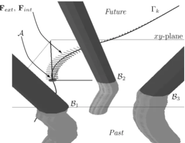
randomly but the model of the future assumes they maintain a constant linear velocity. Fig-ure 2 illustrates in a visual manner howTeddy operates.
Figure 2. Teddy’s principle visualized in a scenario
involving three moving disk obstaclesBi,i=1−3.
The time dimension is pointing upward. The past lies below thexy-plane(the present)and the future lies above. The obstacles are moving randomly, but the model of the future assumes that they maintain a constant linear velocity. The internal and external forces acting upon the nodes of the trajectoryΓkare
represented by vectors.
4.1. “Cutting” Scenario
To emphasize the interest of trajectory defor-mation vs path deformation, a “cutting” sce-nario similar to the one depicted in Figure 1 has been considered first. This scenario was selected because it is problematic for classical path deformation schemes.
Teddy relies upon a number of parameters to operate properly: the repulsion gain kext, the
attraction gain kint and the distance functions
dwtanddst. The two examples presented below
have been selected to illustrate the importance of the distance functiondwton the performance
of Teddy. Recall thatdwt is used to determine
the distance between a trajectory node and the closest obstacle inW×T(cf. subsection 2.3). In both examples, the initial trajectory had a dura-tion of 20s and the discrete trajectory contained 320 nodes. Teddywould run at 28Hz.
For the same scenario, two very different de-formation patterns can be obtained by properly selecting the weightswsandwtin(2). The first
example is obtained by giving more weight to
ws thereby allowing more important spatial
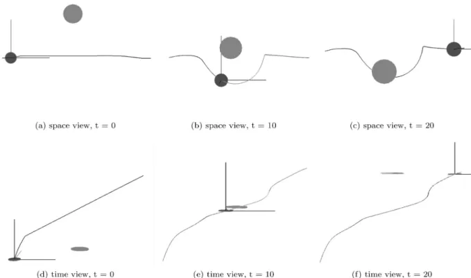
Figure 3.“Cutting” scenario(spatial deformation):Ais moving from the left to the right, the obstacle is moving downwards. The top snapshots depict the path at different time instant(x×yview). The bottom snapshots depict the
velocity profile at the same instants(x×tview).
The second example, on the other hand, is ob-tained by giving more weight towt thereby
al-lowing more important temporal deformations to take place (Figure 4). In this case, A lets the obstacle cross its path before proceeding. The path component of the trajectory is only slightly modified whereas the velocity compo-nent is largely deformed so as to allow A to slow down and stop in order to give way to the obstacle.
These two examples have shown the influence of the choice of the parameters in the final per-formance ofTeddy. They have also illustrated the advantage of trajectory deformation versus path deformation.
4.2. Miscellaneous Scenarios
Afterwards,Teddy was tested on different sce-narios featuring up to 10 obstacles moving ran-domly(their linear velocity change at each time cycle). Three runs with different settings for the weightsws andwtare illustrated in Figures 5 to
7. In Figure 5,wsis the most important thereby
allowing more important spatial deformations to take place. In Figure 6,wtis the most
impor-tant thereby allowing more imporimpor-tant temporal
deformations to take place. In Figure 7,wsand
wt are balanced, both spatial and temporal
de-formations take place. Finally,Teddywas tested on a scenario featuring both fixed and moving obstacles(Figure 8).
4.3. Performances of Teddy
From a complexity point of view, it grows lin-early with the number of nodes and the number of obstacles. Table 1 gives the running time of one deformation cycle for different numbers of nodes and obstacles. These results show the ability of Teddy to operate efficiently even in highly cluttered environments.
number of nodes number of
obstacles 50 100 180 250 320
1 6 11 20 27 35
3 44 48 68 70 73
10 49 88 135 199 229
Figure 4.“Cutting” scenario(temporal deformation):Ais moving from the left to the right, the obstacle is moving downwards. The top snapshots depict the path at different time instant(x×yview). The bottom snapshots depict the
velocity profile at the same instants(x×tview).
Figure 5.Multi-disk scenario(spatial deformation):Ais moving from the bottom-left corner to the top-right corner.
Figure 6.Multi-disk scenario(temporal deformation):
Figure 7.Multi-disk scenario(spatio-temporal deformation):Ais moving from the bottom-left corner to the top-right corner.
5. Conclusion and Future Works
The paper has presentedTeddy, a trajectory de-formation scheme. Given a nominal trajectory reaching a given goal, Teddy deforms it reac-tively in response to updated information about the environment’s obstacles. Teddycan handle robotic systems with arbitrary dynamics. It has been applied to the case of a 2D double inte-grator system and tested in various situations. Because,Teddyexplicitly takes into account in-formation on the future behaviour of the obsta-cles, it is able to handle situations that are prob-lematic for classical path deformation schemes. In the future, it is planned to consider other robotic systems, e.g. differential drive/car-like vehicles, and to further optimizeTeddy. Con-sidering, for instance, that the knowledge about the future behaviour is less reliable in the distant future, it could be interesting to monotonically decrease the influence of the obstacles with re-spect to time. Last but not least,Teddyremains to be integrated within a global navigation archi-tecture and tested on an actual robotic system. It is planned to do so on the architecture and the vehicle presented in Chen et al. (2007).
Acknowledgments
This work was supported by the French Ministry of Defence(DGA Doctoral Grant) and by the European Commission contracts “Cybercars-2 FP6-IST-2004-028062” and “Have-It FP7-IST-2007-212154”.
References
[1] ASARIN, E., DANG, T., FREHSE, G., GIRARD, A., LEGUERNIC, C.ANDMALER, O., Recent progress in continuous and hybrid reachability analysis. In: Proc. of the IEEE Int. Conf. on Computer Aided Control Systems Design, Munich(DE), Oct. 2006. [2] BROCK, OLIVER AND KHATIB, OUSSAMA, Elastic
Strips: A Framework for Motion Generation in Human Environments.The International Journal of Robotics Research21(12), 2002.
[3] CHEN, G., FRAICHARD, TH. AND MARTINEZ-GOMEZ, L., A Real-Time Autonomous Navigation Architecture. In: Proc. of the IFAC Symp. on In-telligent Autonomous Vehicles, Toulouse(FR), Sep. 2007.
[4] KHATIB, M.ANDJAOUNI, H.ANDCHATILA, R.AND LAUMOND, J.P., Dynamic Path Modification for Car-like Nonholonomic Mobile Robots. In: Pro-ceedings of the 1997 IEEE - International Confer-ence on Robotics and Automation, Albuquerque, New Mexico, April, 1997.
[5] KURNIAWATI, H.ANDFRAICHARD, TH., From Path to Trajectory Deformation. In: Proc. of the IEEE-RSJ Int. Conf. on Intelligent Robots and Systems, San Diego, CA(US), Oct. 2007.
[6] LAMIRAUX, F.ANDBONNAFOUS, D.ANDLEFEBVRE, O., Reactive Path Deformation for Nonholonomic Mobile Robots. In: IEEE Trans. on Robotics and Automation, 20(6), Dec. 2004.
[7] LAVALLE, S. M., Planning Algorithms. Cambridge University Press, 2006.
[8] MITCHELL, I., Comparing forward and backward reachability as tools for safety analysis. In: Hybrid Systems: Computation and Control, Lecture Notes in Computer Science 4416, Springer, 2007. [9] QUINLAN, S.ANDKHATIB, O., Elastic Bands:
Con-necting Path Planning and Control. In Proc. of the IEEE Int. Conf. on Robotic and Automation, Atlanta, GA(USA), May, 1993.
[10] YANG, Y.ANDBROCK, B., Elastic Roadmaps: Glob-ally Task-Consistent Motion for Autonomous Mo-bile Manipulation. In: Proc. of the Int. Conf. Ro-botics: Science and Systems, Philadelphia PA(US), Aug. 2006.
Received:November, 2007
Revised:May, 2008
Accepted:July, 2008
Contact address:
Thierry Fraichard INRIA Grenoble Inovall´ee 655 avenue de l’Europe Montbonnot 38 334 Saint Ismier Cedex France e-mail:[email protected]
THIERRYFRAICHARDis a Research Scientist in the INGRIA Grenoble
Rhˆone-Alpes Research Center in France. He does research on mo-tion autonomy for vehicles with a special emphasis on safe navigamo-tion, motion planning(for nonholonomic systems in dynamic environments and in the presence of uncertainty), prediction of the future motion of moving objects, and the design of control architectures for autonomous vehicles. He received his Ph.D(’92)and his Accreditation to Super-vise Research (’06)in Computer Science from the Institut National Polytechnique de Grenoble(INPG), France.