Representing the Arctic in global surface temperature time series of recent climate change

(1)

Representing the Arctic in Global

Surface Temperature Time Series of

Recent Climate Change

PhD in Atmosphere, Oceans and Climate

Department of Meteorology

Emma Dodd

May 2015

(2)

Declaration

I confirm that this is my own work and the use of all material from other sources has been properly and fully acknowledged.

(3)

Acknowledgements

First and foremost I would like to thank my supervisor Prof. Chrisopher Merchant. I have greatly benefited from all the expertise and guidance he has provided throughout my time as a PhD student. Thanks are also due to my other supervisors, both past and present; Nick Rayner, Prof. Simon Tett and Dr Simone Morak. Furthermore I should thank my monitoring committee at the University of Reading and those on my confirmation panel at the University of Edinburgh for pointing out gaps in my knowledge.

I would like to express my gratitude to the many people whom I had the pleasure to meet during the course of my PhD, especially those at the University of Edinburgh, Met Office Hadley Centre, University of Reading, and the EarthTemp Network Workshops. Thank you for your advice, constructive comments, discussions and support. I would like to offer my special thanks to Dr. Colin Morice who provided guidance, insightful discussion, and data in the course of producing my first paper. I am also indebted to Dr. Josefino Comiso and Larry Stock who kindly shared their renormalised monthly AVHRR data.

Lastly some personal thanks. Thank you to my parents, who gave me the freedom to follow my own path, and my friends, for your company. Special thanks are due to my fellow PhD student Emma Knowland for her friendship, support and sympathy. I hope I was able to reciprocate in at least some small way. I would also like to thank all those who keep up the tradition of 11am coffee in ESSC, especially Drs Claire Bulgin, Claire MacIntosh, Kevin Pearson, Jonathan Mittaz and Owen Embury for their interesting conversation on many topics. And finally to my partner John, my deepest heartfelt appreciation for your unwavering support, encouragement and never failing belief in me.

(4)

Abstract

The Arctic is an important region in the study of climate change, but monitoring surface temperatures in this region is challenging, particularly in areas covered by sea ice. Here in situ, satellite and reanalysis data were utilised to investigate whether global warming over recent decades could be better estimated by changing the way the Arctic is treated in calculating global mean temperature. The degree of difference arising from using five different techniques, based on existing temperature anomaly dataset techniques, to esti-mate Arctic SAT anomalies over land and sea ice were investigated using reanalysis data as a testbed. Techniques which interpolated anomalies were found to result in smaller errors than non-interpolating techniques. Kriging techniques provided the smallest errors in anomaly estimates. Similar accuracies were found for anomalies estimated from in situ meteorological station SAT records using a kriging technique. Whether additional data sources, which are not currently utilised in temperature anomaly datasets, would improve estimates of Arctic surface air temperature anomalies was investigated within the reanaly-sis testbed and using in situ data. For the reanalyreanaly-sis study, the additional input anomalies were reanalysis data sampled at certain supplementary data source locations over Arctic land and sea ice areas. For the in situ data study, the additional input anomalies over sea ice were surface temperature anomalies derived from the Advanced Very High Resolution Radiometer satellite instruments. The use of additional data sources, particularly those located in the Arctic Ocean over sea ice or on islands in sparsely observed regions, can lead to substantial improvements in the accuracy of estimated anomalies. Decreases in Root Mean Square Error can be up to 0.2K for Arctic-average anomalies and more than 1K for spatially resolved anomalies. Further improvements in accuracy may be accomplished through the use of other data sources.

(5)

List of Figures

1.1 Annual global mean surface temperature anomaly (K) relative to 1961-1990 from three combined land-surface air and sea surface temperature datasets; the National Oceanic and Atmospheric Administration (NOAA) National Cli-matic Data Center (NCDC) Merged Land-Ocean Surface Temperature Analysis (MLOST, Vose et al. 2012), the HadCRUT4 global temperature anomaly dataset (Morice et al., 2012) produced by the Met Office Hadley Centre and Climatic Research Unit (CRU) of the University of East Anglia, and the National Aero-nautics and Space Administration (NASA) Goddard Institute for Space Studies (GISS) Surface Temperature Analysis (GISTEMP, Hansen et al. 2010). . . 2 1.2 Different surface temperatures. Sea Surface Temperature (SST): at depth,

mea-sured in situ, or of the skin layer, meamea-sured by radiometers on ships or in space; Marine Air Temperature (MAT); Land Surface Temperature (LST); Surface Air Temperature (SAT); Lake Surface Water Temperature (LSWT); Ice Sur-face Temperature (IST). Fig. 1 from Merchant et al. 2013. . . 3 1.3 Map of the locations and length of temperature record of all

sta-tions in the ISTI Stage 3 Merged Recommended Monthly data-bank product (Thorne et al., 2011). Acquired from f tp :

//f tp.ncdc.noaa.gov/pub/data/globaldatabank/monthly/stage3/recommended/plots /merged locations.gif. . . 7 1.4 A map of grid cells where SST is recorded and the total number of observations

in HadSST3 (Kennedy et al., 2011b,c) for 1850, 1960, 1980 and 2011. . . 8 1.5 Image from the National Snow and Ice Date Center (NSIDC) showing the albedo

(α) of open ocean, bare sea ice and sea ice with snow. Acquired from http :

//nsidc.org/cryosphere/seaice/processes/albedo.html(NSIDC, 2013). . . 11 1.6 Arctic sea ice extent from NSIDC as of September 17th 2014.

Sum-mertime daily sea ice extents are also shown for 2010-2014, along with the 1981-2010 average and standard deviations. Acquired from http :

//nsidc.org/arcticseaicenews/2014/09/arctic−minimum−reached/(NSIDC, 2014).. . . 13

(11)

2.1 The annual correlation function in high latitudes produced using the parameters identified by Hansen and Lebedeff 1987 and Rohde et al. 2012. This was the reference correlation function for annual Arctic SAT anomalies. The reference annual correlation length scale was 1570km. . . 37 2.2 The seasonal correlation function in high latitudes based on the correlation

tions identified by Rigor et al. 2000. These were the reference correlation func-tions for monthly Arctic SAT anomalies. The reference monthly correlation length scales were 1020km (spring, autumn, winter) and 710km (summer). . . . 38 2.3 The locations of all Arctic (above 65◦N) meteorological stations in the

GHCN-Mv3.1.0 dataset. . . 39 2.4 The cross correlation of grid-cell annual average anomalies from the grid cell

nearest three station locations (Rowley Island, Hall Beach and Corkudah) with the annual average anomalies for all other ERA-Interim grid cells. Black dots show station locations and black circles show the area which is 1570km distance from each station location. . . 42 2.5 Scatter plot of the correlation between grid cell annual average anomalies from

the grid cell nearest three Arctic station locations (Rowley Island, Hall Beach and Corkudah) with the annual average anomalies for all other ERA-Interim grid cells. The black line gives the polynomial fit to the data and the dashed lines show the reference correlation length scale. . . 42 2.6 The cross correlation of grid-cell annual average anomalies from the grid cell

nearest three station locations (Alert, Nord Ads and Danmarkshavn) with the annual average anomalies for all other ERA-Interim grid cells. Black dots show station locations and black circles show the area which is 1570km distance from each station location. . . 43 2.7 Scatter plot of the correlation between grid cell annual average anomalies from

the grid cell nearest three Arctic station locations (Alert, Nord Ads and Dan-markshavn) with the annual average anomalies for all other ERA-Interim grid cells. The black line gives the polynomial fit to the data and the dashed lines show the reference correlation length scale. . . 43 2.8 Annual reference and ERA-Interim correlation functions. The dashed lines show

the reference correlation length scale. . . 44 2.9 Graph of the correlation value of grid-cell annual average anomalies at 1570km

(the reference correlation length scale) for all station locations above 65◦N with a reference line representing the reference correlation value associated with the correlation length scale. . . 45

(12)

2.10 Panel plot of the cross correlation of grid-cell monthly average anomalies from the grid cell nearest the Tuktoyaktuk, N.W.T station location with the monthly average anomalies for all other ERA-Interim grid cells. Black dots show the station location and the black circles show the area which is 1020km (spring, autumn, winter) or 710km (summer) distance from the station location. . . 46 2.11 Scatter plot of the correlation between grid cell monthly average anomalies from

the grid cell nearest the Tuktoyaktuk, N.W.T station locations with the monthly average anomalies for all other ERA-Interim grid cells. The black line gives the polynomial fit to the data and the dashed lines show the reference correlation length scale. . . 47 2.12 Seasonal reference and monthly ERA-Interim correlation functions. The dashed

lines show the reference correlation length scale. . . 48 2.13 Monthly reference and ERA-Interim correlation functions. The dashed lines

show the reference correlation length scale. . . 49 2.14 Graph of the monthly cross correlation value at 1020km and 710km (summer)

for each station location above 65◦N and the average monthly cross correlation value at these distances across all station locations above 65◦N. Dashed grey lines show the reference correlation value at the distances of interest. . . 49 3.1 The number of stations (a) reporting at least one temperature in each

year, (b) reporting temperatures in all months of each year, and (c) the percentage of grid cells with at least one station reporting within 1200km (‘Fractional Coverage’). . . 53 3.2 The annual Arctic SAT anomaly (K) over land relative to 1961-1990

from several temperature anomaly datasets; Global Historical Climatology Network-Monthly temperature dataset (GHCN-M, Lawrimore et al. 2011), National Aeronautics and Space Administration (NASA) Goddard Insti-tute for Space Studies (GISS) Surface Temperature Analysis (GISTEMP, Hansen et al. 2010), and the Climatic Research Unit of the University of East Anglia and Met Office Hadley Centre land surface temperature anomaly dataset version 4 (CRUTEM4, Jones et al. 2012). The timeseries are produced from the dataset grids using grid boxes north of 65◦N over land and converted to be relative to 1961-1990. The dataset versions used for this figure are GHCN-M.3.2.2.20140729, GISTEMP (downloaded on the 29th July 2014) and CRUTEM4.2.0.0. . . 54 3.3 The locations of all meteorological stations in the CRUTEM4 databank.

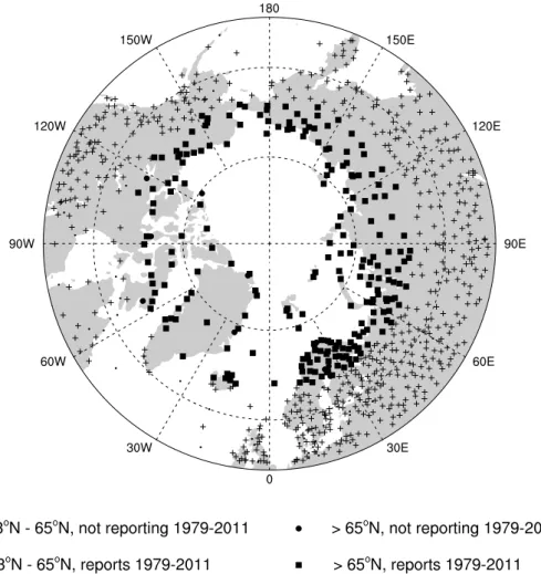
Different markers are used to show the locations of the meteorological sta-tions depending on whether they are above 53◦N or above 65◦N and whether or not they report a single temperature between 1979 and 2011. . . 58

(13)

3.4 A diagram illustrating the creation of an ensemble dataset of input anoma-lies using ERA-Interim data masked according to station coverage between 1850 and 2011. Each ensemble member comprises a set of repeated in-stances of one 12-month year from the period 1979-2011, masked according to the station coverage between 1850 and 2011. . . 59 3.5 Left: time series of annual Arctic-average anomalies between 1979 and

2011 produced using each estimation technique investigated in this study and from reference anomalies. Right: the errors in estimated anomalies relative to the reference anomalies. . . 64 3.6 Timeseries of the errors in estimated monthly Arctic-average anomalies

relative to the reference anomalies between 1979 and 2011 for each esti-mation technique investigated in this study. One representative month for each season is shown. . . 64 3.7 A box-whisker plot of the range, median and lower and upper quartiles of

monthly area-weighted Arctic Surface Air Temperature averaged over land and sea ice from ERA-Interim between 1979 and 2011. A reference line is included at 273.13K. . . 65 3.8 A Taylor Diagram comparing estimated Arctic-average monthly and annual

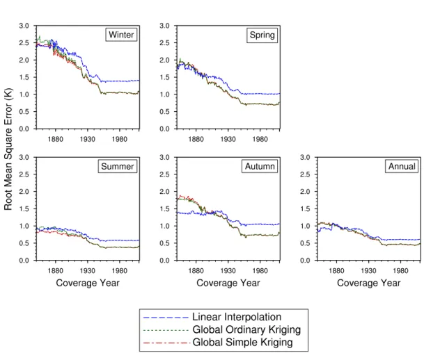
anomalies produced by each estimation technique investigated in this study to the reference anomalies. Each symbol plotted represents a month of the year or the annual value. Cross correlation is shown by the angle with respect to the x-axis. The standard deviations (normalised with respect to the reference standard deviation) can be read from the y-axis. The Root Mean Square Error (K) of the estimated anomalies is proportional to the distance to the point on the x-axis identified as REF (shown by the concentric circles marked 0.25 to 1). The values for July estimated by Not Interpolating and Not Interpolating and Regridding are off the scale of this diagram. . . 66 3.9 The Root Mean Squared Error (K) and Compound Relative Error between

spatially resolved annual Arctic anomalies estimated using the investigated interpolating techniques and reference anomalies in recent decades (1979 - 2011). CRE is a unitless metric where 0 is the best result and higher numbers represent a higher relative error. . . 68 3.10 The area-weighted average of the Root Mean Square Error (K) and

Com-pound Relative Error between estimated spatially resolved Arctic anomalies (estimated using the investigated interpolating techniques) and reference anomalies in recent decades (1979-2011). Left: monthly anomalies. Right: annual anomalies. CRE is a unitless metric where 0 is the best result and higher numbers represent a higher relative error. . . 69

(14)

3.11 The error in annual Arctic-average anomalies estimated by Linearly In-terpolating each year of ERA-Interim anomalies (1979-2011, each year is shown by one line) masked using historical station coverages (1850-2011). Similar graphs for all estimation techniques and seasons are provided in Appendix C. . . 71 3.12 The Root Mean Square Error (K) and Compound Relative Error across

ensemble members (each year of ERA-Interim anomalies 1979-2011) in each historical coverage year for estimated seasonal and annual Arctic-average anomalies. CRE is a unitless metric where 0 is the best result and higher numbers represent a higher relative error. . . 72 3.13 The area weighted Root Mean Square Error (K) for spatially resolved Arctic

anomalies across ensemble members (each year of ERA-Interim anomalies 1979-2011) produced by the investigated interpolating techniques. . . 73 3.14 The mapped Root Mean Square Error (K) across an ensemble of 33 different

years of ERA-Interim data (1979-2011) for spatially resolved annual Arc-tic anomalies produced using Global Ordinary Kriging and Global Simple Kriging for two example historical coverage years (1901, top; 1939, bottom). 74 3.15 The Mean Error (K) for ensemble members (each year of ERA-Interim

anomalies 1979-2011) and the percentage of ensemble members with posi-tive errors in each historical coverage year for estimated seasonal and annual Arctic-average anomalies. Anomalies were estimated using all estimation techniques investigated in this study excluding Not Interpolating. . . 76 3.16 The trend in (top) Mean Error (K) across the ensemble and (bottom) errors

in each ensemble member. Each ensemble member comprises repeated instances of Winter, Spring and Annual Arctic-average anomalies for an individual year (1979-2011, see text for further details) estimated using Global Simple Kriging. . . 78 4.1 The locations of all meteorological stations in the CRUTEM4 databank

(black), and the 63 independent land stations from ISTI (red) that consti-tute the land validation data in this study. Different marker styles are used to show the locations of the meteorological stations depending on whether they are above 53◦N or above 65◦N. All stations had records in the time period of interest (1950-2013). . . 85 4.2 The tracks of each relevant North Pole Drifting Station (1950-2013) and

CRREL IMB (2003-2013). . . 88 4.3 The Root Mean Squaredd(K) between drifting platform temperatures and

estimated anomalies plotted against the average, minimum and maximum number of days observed. NPDS temperatures are compared between 1950 and 2013 and CRREL IMB temperatures are compared between 2003 and 2013. . . 91

(15)

4.4 A scatter plot of the Absolutedd (K) between CRREL IMB temperatures and anomalies estimated using GSK between 2003 and 2013 against the minimum number of days observed. The minimum number of days observed is calculated from the number of observations which contribute to the two monthly average temperature measurements from CRREL IMBs used to create thedd. Two reference lines show 10 and 15 days observed. . . 93 4.5 Monthly average of the Root Mean Square Error (K) and Compound

Rel-ative Error for the reanalysis study (left) and the the Root Mean Square Difference (K) and Compound Relative Difference for the land validation investigation (right). 95% confidence intervals are given in grey. CRD is a unitless metric where 0 is the best result and higher numbers represent a higher relative error. . . 95 4.6 The spatially resolved Root Mean Square Error (K) from the reanalysis

study and the Root Mean Square Difference (K) for each independent land station for several example months. . . 96 4.7 Monthly average of the Root Mean Square dd (K) for the NPDS sea ice

validation data (top), and the Root Mean Square Error (K) for the reanaly-sis study (bottom) calculated across all EASE-Grid cells over sea ice (left), across only grid cells and months present in the validation data (middle, us-ing metrics for random years between 1979 and 2011), and from simulated double differences for the same grid cells, months and years where possible (right, validation data years before 1979 or after 2011 were replaced ran-domly with years within this time period). 95% confidence intervals are given in grey. . . 97 4.8 The monthly Absolutedd (K) between NPDS temperatures and estimated

anomalies estimated using GSK between 1950 and 2013 plotted against the minimum number of days observed. The minimum number of days observed was calculated from the number of daily temperatures which contribute to the two monthly average temperature measurements from NPDS used to calculate the dd statistic. A line shows the minimum required number of days observed in this study. . . 99 4.9 The number of years between 1950 and 2013 where NPDS report for the

whole of each month. . . 100 4.10 Monthly average of the Root Mean Square dd (K) for the CRREL sea ice

validation data (top) and Root Mean Square Error (K) for the reanaly-sis study (bottom); (left) sampled to the same grid cells and months as the validation data using anomalies for random years between 2003 and 2013, (right) simulateddd for the same grid cells, months and years where possible. 95% confidence intervals are given in grey. . . 101

(16)

5.1 The locations of input anomalies for Chapter 3 (black) and additional input anomalies (red) over land between 1979 and 2011. . . 107 5.2 The locations of additional input anomalies over sea ice between 1979 and

2011. . . 108 5.3 A Taylor diagram comparing the monthly and annual Arctic-average

anomaly timeseries produced in the additional land investigation (colour) and from the reanalysis study (black). Each symbol plotted represents a month of the year or the annual value. Cross correlation is shown by the angle with respect to the x-axis. The standard deviations (normalised with respect to the reference standard deviation) can be read from the y-axis. The Root Mean Square Error (K) of the estimated anomalies is propor-tional to the distance to the point on the x-axis identified as REF (shown by the concentric circles marked 0.25 to 1). . . 110 5.4 The change in Root Mean Square Error (K) and Compound Relative

Er-ror for spatially resolved annual SAT anomalies in the Arctic between the additional land data investigation and the reanalysis study. . . 111 5.5 The change in the Root Mean Square Error (K) and Compound Relative

Error between the reanalysis study and the additional land data investi-gation for the Global Ordinary Kriging technique. Maps are plotted for several months of interest for each error metric. . . 113 5.6 The change in the Root Mean Square Error (K) and Compound Relative

Error between the reanalysis study and the additional land data investiga-tion for the Linear Interpolainvestiga-tion technique. Maps are plotted for several months of interest for each error metric. . . 113 5.7 A Taylor diagram comparing the monthly and annual Arctic-average

anomaly timeseries from this additional sea ice investigation (colour) and from the reanalysis study (black). Each symbol plotted represents a month of the year or the annual value. Cross correlation is shown by the angle with respect to the x-axis. The standard deviations (normalised with re-spect to the reference standard deviation) can be read from the y-axis. The Root Mean Square Error (K) of the estimated anomalies is proportional to the distance to the point on the x-axis identified as REF (shown by the concentric circles marked 0.25 to 1). . . 115 5.8 The change in Root Mean Square Error (K) and Compound Relative

Er-ror for spatially resolved annual SAT anomalies in the Arctic between the additional sea ice data investigation and the reanalysis study. . . 116 5.9 The change in the Root Mean Square Error (K) and Compound Relative

Error between the reanalysis study and the additional sea ice data inves-tigation for the Global Ordinary Kriging technique. Maps are plotted for several months of interest for each error metric. . . 117

(17)

5.10 The change in the Root Mean Square Error (K) and Compound Relative Error between the reanalysis study and the additional sea ice data investi-gation for the Linear Interpolation technique. Maps are plotted for several months of interest for each error metric. . . 118 5.11 Area weighted average of the spatially resolved RMSE and CRE from the

reanalysis study and the additional sea ice data investigation. . . 119 6.1 The locations of all meteorological stations in the CRUTEM4 databank.

Different markers are used to show the locations of the meteorological sta-tions depending on whether they are above 53◦N or above 65◦N and whether station normals are available between 1981 and 2004. . . 126 6.2 Spatially resolved calendar monthly average surface temperatures (K) from

the AVHRR dataset of Comiso and Hall 2014, and monthly average surface air temperatures from IABP/POLES (Rigor et al., 2000) and ERA-Interim for the period 1981-2004. . . 129 6.3 The Mean Difference (K) between spatially resolved monthly average

sur-face temperatures from the AVHRR dataset of Comiso and Hall 2014, and monthly average surface air temperatures from IABP/POLES (Rigor et al., 2000) and ERA-Interim between 1981 and 2004. . . 130 6.4 Monthly surface temperature data 1981-2008 from the AVHRR dataset of

Comiso and Hall 2014 compared to the validation data used in this study (from NPDS and other reliable data sources over Arctic sea ice). . . 130 6.5 Monthly temperature timeseries from the AVHRR dataset of Comiso and

Hall 2014 and NPDS observations (both those in the grid cell and those up to 100km away) for the EASE grid cell located at 83.62N, 8.13W compared to the temperature timeseries from a nearby Arctic land-based meteorolog-ical station (within 300km of the grid cell). . . 131 6.6 Monthly temperature timeseries from the AVHRR dataset of Comiso and

Hall 2014 and NPDS observations (both those in the grid cell and those up to 200km away) for the EASE grid cell located at 81.83N, 73.66W compared to the temperature timeseries from a distant Arctic land-based meteorological station (more than 1200km distance from the grid cell). . . 132 6.7 Monthly temperature anomaly timeseries from the AVHRR dataset of

Comiso and Hall 2014 and NPDS observations (both those in the grid cell and those up to 100km away) for the EASE grid cell located at 83.62N, 8.13W compared to the temperature timeseries from a nearby Arctic land-based meteorological station (within 300km of the grid cell). . . 133

(18)

6.8 Monthly temperature timeseries from the AVHRR dataset of Comiso and Hall 2014 and NPDS observations (both those in the grid cell and those up to 200km away) for the EASE grid cell located at 81.83N, 73.66W compared to the temperature timeseries from a distant Arctic land-based meteorological station (more than 1200km distance from the grid cell). . . 134 6.9 The location of AVHRR input surface temperature anomalies (dark grey).

The AVHRR input anomalies are located in grid cells which contain perma-nent sea ice (at least 15% sea ice in all months) in ERA-Interim reanalysis data (gridded to a 100km EASE grid) in the time period 1981-2013. . . . 135 6.10 Monthly Surface Air Temperature data (K) 1981-2004 from the

IABP/POLES dataset compared to the validation data used in this study, both NPDS and other data sources which are not used in the IABP/POLES analysis. . . 138 6.11 Monthly scatter plots of monthly anomalies 1981-2013 from the reference

and AVHRR interpolations compared to validation anomalies. Black mark-ers represent the reference interpolation, red markmark-ers represent the AVHRR interpolation. . . 141 6.12 The Root Mean Square Difference (K) and Compound Relative Difference

between estimated Arctic anomalies, from the reference and the AVHRR interpolations, and validation data 1981-2013. 95% confidence intervals are given for the RMSE from both interpolations. CRE is a unitless metric where 0 is the best result and higher numbers represent a higher relative error. . . 142 6.13 Change in Root Mean Square Difference (K) for several example months

between AVHRR interpolation and reference interpolation monthly esti-mated anomalies for produced. . . 143 6.14 Decadal scatter plots of monthly anomalies (K) from the two interpolations

compared to validation anomalies. A reference line is given showing x=y. The Mean Error and Root Mean Square Error values are given for each decade and for each interpolation. . . 145 C.1 The error in annual Arctic-average anomalies estimated by using Global

Ordinary Kriging on each year of ERA-Interim anomalies (1979-2011, each year is shown by one line) using historical station coverages (1850-2011). . 166 C.2 The error in annual Arctic-average anomalies estimated by using Global

Simple Kriging on each year of ERA-Interim anomalies (1979-2011, each year is shown by one line) using historical station coverages (1850-2011). . 167 C.3 The error in annual Arctic-average anomalies estimated by using the

Bin-ning technique on each year of ERA-Interim anomalies (1979-2011, each year is shown by one line) using historical station coverages (1850-2011). . 168

(19)

C.4 The error in seasonal Arctic-average anomalies estimated by Linearly In-terpolating each year of ERA-Interim anomalies (1979-2011, each year is shown by one line) using historical station coverages (1850-2011). . . 169 C.5 The error in seasonal Arctic-average anomalies estimated by using Global

Ordinary Kriging on each year of ERA-Interim anomalies (1979-2011, each year is shown by one line) using historical station coverages (1850-2011). . 170 C.6 The error in seasonal Arctic-average anomalies estimated by using Global

Simple Kriging on each year of ERA-Interim anomalies (1979-2011, each year is shown by one line) using historical station coverages (1850-2011). . 171 C.7 The error in seasonal Arctic-average anomalies estimated by using the

Bin-ning technique on each year of ERA-Interim anomalies (1979-2011, each year is shown by one line) using historical station coverages (1850-2011). . 172

(20)

List of Tables

2.1 A summary of the performance of currently available reanalyses for Arctic temperatures, including information on whether the comparison data for each study is independent or assimilated into the reanalysis. Acronyms used in this table are: Decadal (D), Annual (A), Seasonal (SNL), Monthly (M), Spatial (SPA) and Timeseries (TS). . . 32 D.1 Potentially suitable sources of further SAT data over sea ice areas in the

(21)

Chapter 1 Introduction

1.1 Recent Global Climate Change

Warming of the Earth’s land surface was first noted by Callendar 1938, who used temper-ature observations from 200 meteorological stations to demonstrate that air tempertemper-atures over land had increased in the 50 years prior to that study (Hawkins and Jones, 2013). Subsequently, climate change over all surfaces of the Earth has become a major topic in contemporary scientific research. Many researchers and organisations are working to quantify post-industrialisation climate change both globally and regionally, assess how fast it is happening and what the consequences will be.

Currently it is estimated that global mean surface temperatures have risen by around 0.8K between 1850 and 2014 (Berkeley Earth, 2014; Hansen et al., 2010; Hartmann et al., 2013; Ishii et al., 2005; Jones et al., 2012; Kaplan et al., 1998; Kennedy et al., 2011b; Kent et al., 2013; Lawrimore et al., 2011; Morice et al., 2012; Muller et al., 2013; Rayner et al., 2003; Rohde et al., 2013b; Smith et al., 2008; Vose et al., 2012). This warming in global mean surface temperatures is illustrated in Figure 1.1, which shows the annual anoma-lies of global land-surface temperatures between 1880 to 2012 from three temperature anomaly datasets. The datasets differ slightly in their annual variations due to structural uncertainty (the uncertainty arising from the choice of methodology) but show a common trend of rising global average surface temperatures. This trend is also noted in regional surface temperature datasets (e.g. Menne et al., 2009; Vincent et al., 2012).

Consistent with the observed increases in surface temperatures other changes have been observed including: warming of the oceans and atmosphere, decreasing snow cover, decreases in Arctic sea ice thickness and extent, almost global reductions in glacier and ice sheet mass and extent, and sea level rise (Intergovernmental Panel on Climate Change, 2013). The Intergovernmental Panel on Climate Change (IPCC) has concluded in its Fifth Assessment Report (AR5) that “Warming of the climate system is unequivocal, and since the 1950s, many of the observed changes are unprecedented over decades to millennia” (IPCC, 2013). This report also concluded that “It is extremely likely that human influence has been the dominant cause of the observed warming since the

(22)

mid-Figure 1.1: Annual global mean surface temperature anomaly (K) relative to 1961-1990 from three combined land-surface air and sea surface temperature datasets; the National Oceanic and Atmospheric Administration (NOAA) National Climatic Data Center (NCDC) Merged Land-Ocean Surface Temperature Analysis (MLOST, Vose et al. 2012), the HadCRUT4 global temperature anomaly dataset (Morice et al., 2012) produced by the Met Office Hadley Centre and Climatic Research Unit (CRU) of the University of East Anglia, and the National Aero-nautics and Space Administration (NASA) Goddard Institute for Space Studies (GISS) Surface Temperature Analysis (GISTEMP, Hansen et al. 2010).

20th _{century” (IPCC, 2013) as a result of the increase in atmospheric concentrations of} greenhouse gases since 1750.

1.2 Monitoring Recent Climate Change

Post-industrialisation changes in climate are often monitored using timeseries of global and regional mean surface temperatures, which are temperatures measured at, or near, the surface of the Earth. Timeseries of global and regional mean Surface Air Temperature (SAT) anomalies are one of the main metrics used to estimate recent climate change. SATs measured at meteorological stations are largely used to generate these timeseries over land and sea ice. For most of the ocean Sea Surface Temperatures (SSTs), collected in situ or derived from satellite instruments, are used. This section provides an overview of the types of surface temperatures most relevant to this thesis and how these temperatures are observed; some of the biases, quality control and data coverage issues associated with surface temperature records; and how surface temperatures are currently utilised to produce datasets and timeseries of global mean surface temperature change.

1.2.1 Surface Temperatures

There are various types of surface temperature that can be employed to monitor surface temperature change and therefore changes in climate. Surface temperatures are often

(23)

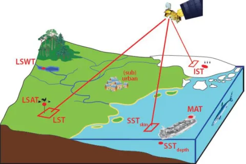
differentiated by the type of surface they are associated with (e.g. ocean, land, ice) and/or the height, or depth, at which they are measured as illustrated in Figure 1.2. These temperatures are measured from sensors on various different platforms. They may be measured in situ or derived from satellite sensor measurements. Surface temperatures, such as those in Figure 1.2, which could be used to monitor changes in climate in the Arctic (those most relevant for this thesis) are discussed here along with the platforms used to measure them.

Figure 1.2: Different surface temperatures. Sea Surface Temperature (SST): at depth, mea-sured in situ, or of the skin layer, meamea-sured by radiometers on ships or in space; Marine Air Temperature (MAT); Land Surface Temperature (LST); Surface Air Temperature (SAT); Lake Surface Water Temperature (LSWT); Ice Surface Temperature (IST). Fig. 1 from Merchant et al. 2013.

1.2.1.1 Surface Air Temperature

Of the temperatures illustrated in Figure 1.2, one of the most commonly used to measure global and regional mean surface temperature change is the SAT. SATs measured in situ are generally used to monitor global temperature change over land and sea ice areas. They provide the longest running instrumental records of temperature in the world; the Met Office Hadley Centre Central England Temperature (HadCET) dataset provides monthly temperatures back to 1659 (Manley, 1953). SAT is generally measured by shielded ther-mometers or temperature sensors at a height of between 1.25 and 2.0m above the surface of the Earth. These sensors may be placed in a Stevenson screen or mounted on other measuring platforms such as a meteorological tower. In situ SATs over areas of sea ice are measured from drifting buoys and drifting ice stations (e.g. Polashenski et al., 2011; Rigor et al., 2000; Uttal et al., 2002). As SATs are measured at around 1.5m height they are influenced by sensible and latent heat exchanges with the atmosphere and surface of the Earth, radiation emitted from the Earth’s surface, solar radiation, and lateral advection.

(24)

Radiometric surface temperatures from satellite instruments can be related to SATs, but are not generally utilised at present for monitoring surface temperature change.

1.2.1.2 Sea Surface Temperature and Marine Air Temperature

Sea Surface Temperature (SST) and Marine Air Temperature (MAT) are the types of temperatures used to monitor global temperature change over the oceans. SST is a measurement of the water temperature close to the surface of the ocean, up to several metres below the surface (Kennedy et al., 2011c). MAT is a measurement of the air temperature above the surface of the ocean. Both SST and MAT are measured from in situ temperature sensors on platforms such as ships, oceanographic stations, moored buoys, drifting buoys and research vessels (Kent and Taylor, 2006; Kent et al., 2013; Kennedy et al., 2011b; Woodruff et al., 2011). In common with SATs, SSTs and MATs provide a long temperature record; for example, the Met Office Hadley Centre’s sea surface temperature dataset version 3 (HadSST3) extends from 1850 to present (Kennedy et al., 2011b,c).

SST anomalies are more frequently employed to monitor global temperature change than MAT anomalies as SST measurements are thought to be more homogeneous (Rayner et al., 2003). Records of MAT change are almost exclusively produced using Night-time only Marine Air Temperature (NMAT) (Kent et al., 2013; Rayner et al., 2003). Daytime MATs are often affected by direct or indirect solar heating, although corrected daytime MAT records are available (Berry and Kent, 2009). MATs are also affected by biases resulting from increasing observing platform height as the average height of ship’s decks have increased over time (Kent et al., 2013; Rayner et al., 2003). Additionally, SST observations are more plentiful (Rayner et al., 2003). As a result SSTs are generally used to monitor global temperature change over the oceans as a proxy for MAT. Air temperatures are significantly influenced by exchanges of heat and radiation from the surface of the Earth so SST anomalies can be expected to agree well with MAT anomalies, at least on seasonal and longer time-scales, as a result of the thermal lag of the oceans. SST anomalies have been compared to NMAT anomalies and this has been confirmed (Rayner et al., 2003; Kent et al., 2013). Nonetheless, MAT datasets are still produced and used to monitor post-industrialisation climate change (Berry and Kent, 2009; Hartmann et al., 2013; Kent et al., 2013).

SSTs can additionally be derived from infrared or microwave radiometers flown on satellites such as the AVHRR (Advanced Very High Resolution Radiometer, e.g. Casey et al. 2010), ATSR (Along Track Scanning Radiometer, e.g. Merchant et al. 2012) and AMSR-E (Advanced Microwave Scanning Radiometer for the Earth observing system, e.g. Wentz and Meissner 2000). Satellite instruments provide relatively detailed obser-vations, with a greater spatial coverage, of the radiometric temperature of water (and ice, see Section 1.2.1.3) surfaces (Merchant et al., 2013). Satellite radiometers observe brightness temperatures in one or more wavelengths for the surface skin of the ocean

(25)

(within 1 mm of the ocean surface). The SST is derived from brightness temperatures using retrieval schemes employing either coefficients (e.g. Embury and Merchant, 2012; Wentz and Meissner, 2000, 2007) or optimal estimation (e.g. Merchant et al., 2008). SSTs derived from infrared instruments are more commonly used than those from microwave instruments as their spatial resolution is higher. However, infrared instruments cannot collect temperature information in the presence of cloud cover and their SST retrieval schemes also have to account for factors such as viewing angle and aerosols (Embury and Merchant, 2012; Merchant et al., 2008). Microwave derived brightness temperatures are negligibly affected by clouds, but the microwave SST retrieval schemes do have to account for factors including sea surface roughness, salinity and precipitation (Wentz et al., 2000; Wentz and Meissner, 2000, 2007). It should be noted that, when comparing satellite derived SST and in situ SSTs, a skin to bulk SST conversion will also need to be applied.

1.2.1.3 Ice Surface Temperature

Ice Surface Temperatures (IST) are a measurement of the temperature of the surface layer of ice or snow. ISTs are not often used to monitor surface temperature change, but could provide a useful temperature record in the sparsely observed polar regions. ISTs could be used as a proxy for SATs over ice and snow, similar to the way SST is used as a proxy for MATs. ISTs can be derived from in situ sensors on platforms as radiometers (Scambos et al., 2006) and Ice Mass Balance Buoys (IMBs, Polashenski et al. e.g. 2011; Richter-Menge et al. e.g. 2006). However, currently the majority of IST observations come from satellites - derived either from microwave or infrared radiometers.

As with SSTs, ISTs are derived from brightness temperatures retrieved from satellite radiometers (e.g. Comiso et al., 2003; Hall et al., 2004). Microwave radiometers are not affected by cloud cover or polar darkness and therefore are useful for monitoring snow and ice temperature change. However, microwaves penetrate into ice and snow beyond the surface, so temperature information derived from these sensors is not easily relatable to IST, and their relatively coarse spatial resolution limits their utility for studies of sea ice temperatures (Hall et al., 2004). Therefore, IST is generally estimated using infrared instruments such as AVHRR (Key and Haefliger, 1992; Lindsay and Rothrock, 1994) and the MODerate-resolution Imaging Spectroradiometer (MODIS, Hall et al. 2004).

1.2.1.4 Lower Tropospheric Temperature

Lower Tropospheric Temperature (TLT) is the temperature of the lower part of the tro-posphere; from the surface to around 3km altitude (Hartmann et al., 2013). In common with IST, upper air temperatures are not as commonly utilised as observations of SAT and SST for monitoring global temperature changes but could provide a useful temper-ature record in sparsely observed areas (Chapters 5). TLT datasets derived from in situ and satellite sources have been used to monitor upper air temperature change (e.g. Mears and Wentz, 2009), have been included in datasets of surface temperature change (Cowtan

(26)

and Way, 2014), and are included in the IPCC AR5 report (Hartmann et al., 2013). TLT can be measured by in situ platforms (radiosondes or rawinsondes, Thorne et al. 2005) and estimated from satellite instruments such as the Microwave Sounding Unit (MSU, Christy et al. 2003; Mears and Wentz 2009). Satellite estimates of TLT are es-timated from brightness temperatures up to 12.5km height, which are heavily weighted to be more representative of the temperature of the troposphere below 3km (Hartmann et al., 2013; Mears and Wentz, 2009). As TLT observations include the temperature of the atmospheric boundary layer, where temperatures are influenced by exchanges of heat and radiation from the surface of the Earth, the temperature trends and short term variations in upper air temperatures are highly correlated with those at the surface but are of a greater amplitude (Hartmann et al., 2013).

1.2.2 Biases, Quality Control and Incomplete Data Coverage

There are many types of surface temperature records which can be used to monitor recent climate change. However, measurements of surface temperatures are not consistent in space and time. They are subject to biases, quality issues, and may be spatially and temporally sparse.

SAT and SST data have been collected using various methods, instruments and plat-forms since records began in the 1800s (e.g. Folland and Parker, 1995; Kennedy et al., 2011b,c; Kent and Taylor, 2006; Kent and Kaplan, 2006; Trewin, 2010). Other changes have also occurred such as: urbanisation (Parker, 2010; Hansen et al., 2010; Menne et al., 2009; Trewin, 2010); increasing average ship speed (impacting engine room intake and hull contact sensor SST measurements, Kennedy et al. 2011c); land use and land cover change (Trewin, 2010); and the movement, addition or discontinuation of meteorological stations (Menne et al., 2009; Trewin, 2010). These changes result in time-varying biases which are not consistent temporally or spatially (Kent and Taylor, 2006; Trewin, 2010). Such changes may also not have been recorded adequately, leading to uncertainty in the measurements.

Additionally, temperature data coverage is not consistent across the globe. Figure 1.3 shows the location and length of record of all land-based meteorological stations in the In-ternational Surface Temperature Initiative (ISTI) Stage 3 Merged Recommended Monthly databank product (Thorne et al., 2011). The databank is a merged collation of all station records provided for the ISTI global land surface databank project. As illustrated in Fig-ure 1.3, meteorological stations are not evenly distributed across land areas. Some areas, such as North America, are relatively densely populated with stations whilst in others, such as the Arctic, station coverage is sparse. Meteorological station coverage can also be temporally sparse. For example, Figure 1.3 shows that North America has many stations which report for 100 years or more whereas in Antarctica many stations report for 25 years or fewer. Figure 1.4 shows the total number of in situ observations of SST in 1850, 1960, 1980 and 2011 from HadSST3 (Kennedy et al., 2011b,c). Some ocean areas, such

(27)

as the North Atlantic are relatively well observed in most time periods whereas others, such as the Southern Ocean are poorly observed (Figure 1.4). The areas observed and numbers of observations also change temporally, and there are fewer observations earlier in the temperature record (Kennedy et al., 2011c; Rayner et al., 2006). SST observa-tions derived from satellite measurements are more spatially complete than in situ SST observations. However, satellite derived SST observations are not temporally or spatially complete. Thermal infrared observations cannot be used when clouds are present and satellite SST records do not extend as far back in time as in situ measurements. Incom-plete temporal and/or spatial coverage in both SAT and SST observations can lead to biases and uncertainties in temperature timeseries (Cowtan and Way, 2014; Rohde, 2013).

Figure 1.3: Map of the locations and length of temperature record of all stations in the ISTI Stage 3 Merged Recommended Monthly databank product (Thorne et al., 2011). Acquired from

f tp : //f tp.ncdc.noaa.gov/pub/data/globaldatabank/monthly/stage3/recommended/plots /merged locations.gif.

Lastly, temperature records are also affected by quality control issues and systematic uncertainties including, but not limited to: problems with instrumentation (Rigor et al., 2000); quality of station siting (Fall et al., 2011; Trewin, 2010); solar heating effects (Kent and Kaplan, 2006; Kent et al., 2013; Trewin, 2010); data imprecision (temperatures may be recorded at a lower precision than WMO standards recommend, Trewin 2010); and precision changes (Trewin, 2010). There also may be uncertainties resulting from random effects (Kent and Challenor, 2006).

(28)

Figure 1.4: A map of grid cells where SST is recorded and the total number of observations in HadSST3 (Kennedy et al., 2011b,c) for 1850, 1960, 1980 and 2011.

1.2.3 Surface

Temperature

Timeseries

of

Recent

Climate

Change

Surface temperature measurements may be sparse, both temporally and spatially, as well as subject to various inhomogeneities, errors and uncertainties. To exclude these non-climatic variations in temperatures from estimates of actual climate change there are many different techniques, methods and adjustments that can be employed. As a result many different groups generate datasets of SAT anomalies using various techniques from a subset of the available surface temperature records (e.g. Berkeley Earth, 2014; Hansen et al., 2010; Morice et al., 2012; Vose et al., 2012).

Different SAT anomaly datasets have different quality control and bias adjustment methods. Some datasets largely utilise data which have been quality controlled and adjusted by other organisations. The National Aeronautics and Space Administration (NASA) Goddard Institute for Space Studies (GISS) Surface Temperature Analysis, also known as GISTEMP, uses adjusted Global Historical Climatology Network - Monthly tem-perature dataset version 3 (GHCN-Mv3) over land, along with some additional data, and the Extended Reconstructed Sea Surface Temperature dataset version 3b (ERSSTv3b, Smith et al. 2008) over the ocean (GISS, 2014; Hansen et al., 2010). GISTEMP addi-tionally employ their own urbanisation adjustment based on satellite data (Hansen et al., 2010). The CRUTEM4 land surface temperature anomaly dataset (produced by the Cli-matic Research Unit of the University of East Anglia and the Met Office Hadley Centre)

(29)

mainly utilises homogenised temperature records provided by national meteorological ser-vices (Jones et al., 2012). For remaining records, comparisons are made with neighbouring stations and adjustments are made accordingly (Jones et al., 2012). Some datasets use metadata to identify and adjust temperature records. For example, HadSST3 uses meta-data to adjust record according to the measuring platform and methods used (Kennedy et al., 2011c). Finally, some datasets adjust temperature records without the use of metadata. The Berkeley Earth Surface Temperature dataset uses a method they call the ‘scalpel’ to identify large discontinuities in single station records (Rohde et al., 2013a, 2012). The records are then split at these points to create two separate record sections. Any adjustments to the records occur automatically as part of the statistical techniques they employ to produce their dataset (Berkeley Earth, 2014; Rohde et al., 2013a, 2012).

Different techniques are also employed to quantify surface temperature changes from records that are not globally or temporally complete. In situ temperature measurements can be used exclusively without spatial infilling of data. This technique is employed to create the HadCRUT4 global temperature anomaly dataset (Morice et al., 2012) which is produced by the Met Office Hadley Centre from a combination of CRUTEM4 over land and HadSST3 over ocean areas. Any grid boxes which do not have available in situ data are empty in these datasets for the time periods in which SSTs or SATs are unavailable (Morice et al., 2012). Some datasets interpolate and extrapolate surface temperatures. GISTEMP is a combination of linearly interpolated and extrapolated SAT data over land and sea ice, and SST data infilled using statistical methods over the ocean. SAT anomalies are interpolated between stations and extrapolated up to 1200km into land and sea ice regions with no measurements (Hansen et al., 2010; Lawrimore et al., 2011). ERSSTv3 is produced by combining the outputs of low- and high- frequency analyses, which derive decadal and seasonal to interannual SST variations respectively (Smith and Reynolds, 2003, 2004, 2005; Smith et al., 2008). The Berkeley Earth Surface Temperature dataset method uses temperature records from many pre-existing datasets and statistical techniques to produce a globally complete estimate of temperature anomalies over land and ocean areas (Berkeley Earth, 2014; Rohde et al., 2013a,b, 2012). It utilises all available data records over land; the other datasets discussed here require records for which a reference ‘normal’ can be produced to calculate temperature anomalies. A recent update to the dataset adds HadSST ocean data to the Berkeley land-area dataset and extrapolates SAT data from the land-area dataset over sea ice (Berkeley Earth, 2014). Finally, some datasets such as MLOST employ both interpolation and extrapolation with exclusion of data (Vose et al., 2012). MLOST utilises homogenised GHCN-Mv3 meteorological station data for SAT anomalies and ERSSTv3b for SST anomalies (Smith and Reynolds, 2005; Smith et al., 2008; Vose et al., 2012). The SAT data from GHCN-Mv3 are analysed using the same low- and high- frequency analysis employed for ERSSTv3b (Smith and Reynolds, 2005). Areas where data are determined to be insufficient are excluded from the low- and high- frequency analyses (Vose et al., 2012).

(30)

Finally it should be noted that there may also be differences in how each dataset produces temperature anomalies from temperature records. Many datasets use the Cli-mate Anomaly Method (CAM) which uses a typically 30 year reference period to calculate temperature anomalies. Datasets may choose different climatology periods, however; Had-CRUT4 uses 1961-90, Berkeley Earth and GISTEMP use 1951-1980 (Hansen et al., 2010; Morice et al., 2012; Rohde et al., 2013a). Other datasets and dataset versions have used anomaly methods such as the Reference Station Method (RSM) (Hansen and Lebedeff, 1987) and the First Difference Method (FDM) (Peterson et al., 1998).

Despite the structural uncertainty arising from the diversity of techniques used at each stage in producing estimates of recent surface temperature changes, the timeseries pro-duced from temperature anomaly datasets largely result in similar post-industrialisation climate change trends as noted in Section 1.1 and illustrated in Figure 1.1. There is a relatively low impact of differences in methods on trends in global surface temperature timeseries. But, what are the impacts of choices of data and methodology on Arctic surface temperature anomalies? How should these datasets incorporate the appropriate contribution to global and regional-average temperature anomalies of the sea-ice regions of the Arctic Ocean?

1.3 The Importance of the Arctic

The Arctic is an important region in the study of climate change because of expected and observed changes in this region. Temperature changes are predicted, and observed, to be more rapid in the Arctic because of Arctic amplification. However, monitoring Arctic temperature change is difficult, particularly in areas covered by sea ice for all or part of the year. This is because in situ measurements of Arctic surface temperatures are sparse and the records are often short. In addition, utilising SAT records collected in this region can be challenging (Chapter 4). Here Arctic amplification is discussed, the various changes associated with climate change in the Arctic are described, and how Arctic surface temperature changes are currently monitored is outlined.

1.3.1 Arctic Amplification

Arctic amplification occurs as a result of various processes, feedback effects and charac-teristics of the Arctic region. The most notable of these processes is the albedo effect (Serreze and Barry, 2011). As temperatures increase and snow, ice and sea ice melt, darker surfaces (land, vegetation and ocean) are exposed which have a lower albedo and absorb more solar energy (illustrated in Figure 1.5). This lowering of surface albedo and corresponding increase in solar radiation absorption causes increased warming, which melts more snow and ice to expose darker surfaces, and so on in a positive feedback loop called the albedo effect. Albedo changes may also result from soot deposits on snow and other feedback effects may arise from causes such as changes in cloud cover and water

(31)

vapour content (Serreze and Barry, 2011).

Figure 1.5: Image from the National Snow and Ice Date Center (NSIDC) showing the albedo (α) of open ocean, bare sea ice and sea ice with snow. Acquired from http :

//nsidc.org/cryosphere/seaice/processes/albedo.html (NSIDC, 2013).

The following characteristics of the Arctic region can also lead to Arctic Amplification. In the Arctic a larger fraction of energy received at the surface goes into warming compared to areas such as the tropics where more energy goes into evaporation. Therefore a larger fraction of the extra energy received as a result of increasing concentrations of greenhouse gases will go into warming the region compared to other areas of the globe (ACIA, 2005). Also, the atmospheric layer that has to warm in the Arctic in order to warm the surface is much shallower than in the tropics (ACIA, 2005). In addition, because heat is transported to the Arctic by the atmosphere and oceans, alterations in their circulation patterns may increase (or decrease) warming in the Arctic region (ACIA, 2005; Anisimov et al., 2007). Furthermore, it is important to note that the processes and consequences of Arctic amplification will not be confined to the Arctic; there will be global implications. Loss of surface reflectivity in the Arctic will accelerate warming at the global scale, and changes in circulation patterns may increase (or decrease) warming globally (ACIA, 2005).

1.3.2 Arctic Surface Temperature Change

Currently it is estimated that Arctic mean surface temperatures over land have risen by around 3.0K between 1880 and 2012 (see Figure 3.2 of this thesis). This is more than double the warming seen for global mean surface temperatures (Figure 1.1) and is significant enough to affect global mean surface temperature estimates when large areas of the Arctic are excluded from temperature anomaly datasets (Cowtan and Way, 2014; Kennedy et al., 2011a). The area above the Arctic circle covers about 6% of the global area, so if we assume a warming of 3.0K for the Arctic region as a whole this would lead to a warming of global temperatures by 0.18K. This is 20% of the increase in global mean surface temperatures between 1850 and 2014.

(32)

1.3.3 Other Changes in the Arctic Associated with Climate

Change

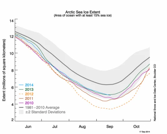
In addition to increasing Arctic surface temperatures over land, many other changes associated with climate change are already being recorded in this region. These changes include rising sea, soil, ice and permafrost temperatures (Comiso, 2001, 2006; Hinzman et al., 2005); warmer and shorter winters (Serreze et al., 2000); increasing length of melt season and area of melt (Comiso, 2006); increasing precipitation and changes in precipitation type (Serreze et al., 2000); decreasing snow cover (Callaghan et al., 2011; Serreze et al., 2000); thawing permafrost (Hinzman et al., 2005; Serreze et al., 2000); changing wind patterns (ACIA, 2005; Anisimov et al., 2007); changes in cloud cover and atmospheric pressure (Comiso, 2001; Przybylak et al., 2013; Serreze et al., 2000); increasing discharge from Arctic draining rivers (Hinzman et al., 2005); decreasing and thinning lake and river ice (Hinzman et al., 2005); more frequent wildfires (ACIA, 2005; Anisimov et al., 2007) and shifting vegetation (Hinzman et al., 2005; Serreze et al., 2000). Sea ice cover has also seen major changes in recent years. The September sea ice extent (the annual minimum extent) has been decreasing by around 13% each decade since satellite records began in 1979 (Perovich et al., 2014). Figure 1.6 shows the Arctic sea ice extent as of September 17th 2014, summertime daily ice extent data for 2010-2014, and the 1981-2010 average and standard deviations (NSIDC, 2014). The 2012 melt season broke the previous record for minimum sea ice extent, set in 2007, before the end of the melt season and as of September 5th_{2012 it was already below 4 million square kilometres} in extent (NSIDC, 2012b; Parkinson and Comiso, 2013). The sea ice extent minimum for 2012 was reached on September 13th _{at 3.40 million square kilometres (NSIDC, 2012a;} Parkinson and Comiso, 2013). The 2013 and 2014 melt seasons have been nearer the 1981-2010 average as shown in Figure 1.6. Less ice is surviving the summer melt so multi-year ice is decreasing (Comiso, 2012; Kwok, 2007; Maslanik et al., 2007; Nghiem et al., 2007; Parkinson and Comiso, 2013; Polyakov et al., 2012). There is also evidence that sea ice in the Arctic is thinning and decreasing in volume (e.g. Kwok et al., 2009; Maslanik et al., 2007; Parkinson and Comiso, 2013). Some studies have indicated that the Arctic will have a sea ice free summer within 30 years (Overland and Wang, 2013; Wang and Overland, 2009). As the Arctic warms and sea ice decreases there is greater access for ships. Already ship traffic is increasing due to tourism and the development of natural resources such as gas, oil, and boreal forest resources (Brigham, 2011; Cressey, 2011; Kullerud, 2011). This leads to increased risk of pollution and oil spills as well as concerns about safety for people, the Arctic environment and the ships that are in these waters (Brigham, 2011). There are also political issues as countries try to lay claim to Arctic resources exposed by the retreating ice (Cressey, 2011). As sea ice extent decreases and the sea ice thins the difficulty of deploying and maintaining manned and unmanned measuring platforms will increase. These changes also shorten the length of time these sensors can operate on ice. This increases the already difficult task of monitoring temperature changes using in situ

(33)

data in sea ice regions.

Figure 1.6: Arctic sea ice extent from NSIDC as of September 17th 2014. Summertime daily sea ice extents are also shown for 2010-2014, along with the 1981-2010 average and standard deviations. Acquired fromhttp ://nsidc.org/arcticseaicenews/2014/09/arctic−minimum−

reached/(NSIDC, 2014).

Furthermore, changes in the Arctic do not just have an impact locally or regionally but also globally. In addition to the impacts of accelerated warming of the Arctic atmo-sphere both regionally and globally, greenhouse gas emissions may increase from the Arctic due to permafrost warming and the release of methane hydrates (ACIA, 2005; Anisimov et al., 2007). These emissions add to the greenhouse gas concentration in the Earth’s atmosphere. Increases in glacial melt, ice sheet melt, ice cap melt and river runoff will contribute to sea level rise which will flood low-lying land. For example, the Greenland Ice Sheet is estimated to have contributed around 0.5mm per year to global sea level rise between 2002 and 2011 (Church et al., 2013; Hanna et al., 2013). This increase in melt will alter the freshwater budget of the Arctic which may affect ocean circulation (ACIA, 2005; Anisimov et al., 2007). There will also be other global impacts resulting from Arctic warming such as changes in animal diversity, ranges and distribution (ACIA, 2005). It is therefore important to monitor and quantify the changes that are happening in the Arctic. But, as the Arctic warms and sea ice extent and thickness decrease how should we monitor the temperature changes occurring in these dynamic and rapidly changing areas?

(34)

1.3.4 Monitoring Arctic Arctic Surface Temperature Change

As we have seen, monitoring climate change in the Arctic region is important because of expected and observed changes in this region. But, in situ measurements of Arctic surface temperatures, particularly in areas covered by sea ice for all or part of the year, are sparse and the records are often short. The sparseness of temperature data for the Arctic is noted as an issue by many researchers as it introduces uncertainty to the calculation of average temperature changes in this region (e.g. Cowtan and Way, 2014; Jones et al., 2012; Parker et al., 2009; Pielke et al., 2007). It is often difficult to assess how temperatures are changing in this region as well as where current climate trends fit in a long term perspective (Bromwich et al., 2007). Also, low density measurements make it hard to separate local changes from regional or continental ones (Bromwich et al., 2007). As described in Section 1.2.3 there are many different techniques and methods that are employed to quantify surface temperature changes from records that are not spatially or temporally complete. There are therefore many different techniques and methods used to quantify SAT changes over the Arctic from sparse in situ measurements.

The majority of currently available temperature anomaly datasets estimate Arctic temperature change using SAT and SST measurements. These surface temperature mea-surements are used exclusively and/or interpolated and extrapolated using various tech-niques. Datasets which use available in situ temperature measurements exclusively, for example many of the Met Office Hadley Centre temperature anomaly datasets such as HadCRUT4 (Morice et al., 2012) and HadSST3 (Kennedy et al., 2011b,c), do not spatially infill data. This means that large areas of the Arctic are unrepresented in these datasets even with recent updates to the datasets (Kennedy et al., 2011b; Morice et al., 2012). Temperature anomaly datasets which interpolate and extrapolate temperatures, such as the GISTEMP (Hansen et al., 2010; Lawrimore et al., 2011) and Berkeley Earth (Berke-ley Earth, 2014; Muller et al., 2013; Rohde et al., 2013a, 2012) analyses, are spatially complete for the Arctic. Sea ice areas in both of these datasets are treated as if they were land areas with a geographical area which changes over time with sea ice extent. MLOST employs both spatial infilling and the exclusion of data. Temperature data are interpolated where possible and excluded where data are determined to be insufficient to interpolate temperature anomalies (less than 20% sampling), the target is polar land (above 75◦N) with no data in the month of interest, and/or more than half the grid box is classified as sea ice (Vose et al., 2012). Therefore large areas of the Arctic are excluded (Vose et al., 2012). Temperatures over areas of Arctic sea ice are therefore either excluded or estimated by interpolating and extrapolating SATs over sea ice areas from land-based SAT sources. These datasets deal with the paucity of Arctic temperature data from tradi-tional observations in various different ways. However, this sparseness of data also makes it difficult to investigate the impact of choices of data and methodology on Arctic surface temperature anomalies. How should Arctic sea ice areas be treated in global and regional averages of surface temperatures?