TRAFFIC
LIGHT
DISPERSION
CONTROL
BASED
ON
DEEP
REINFORCEMENT
LEARNING
Bryan Chuab,KamarulafizamIsmaila,b,*, Fazila Mohd Zawawib, Nur Safwati Mohd Norb
a Media and Game Innovation Center of Excellence
bSchool of Mechanical Engineering,
UniversitiTeknologi Malaysia, 81200 Skudai, Johor Bahru, Malaysia
Article history Received 21 November 2019 Received in revised form
27 September 2019 Accepted 31 December 2019
Published Online 31 December 2019
*Corresponding author [email protected]
A
BSTRACTThe current traffic light controls are ineffective and causes a handful of problems such as congestion and pollution. This study investigates the application of deep reinforcement learning on traffic control systems to minimize congestion at traffic intersection. The traffic data from Pulai Perdana, Skudai, Johor Intersection was extracted, analysed and simulated based on the Poisson Distribution, using a simulator, Simulation of Urban Mobility (SUMO). In this research, we proposed a deep reinforcement learning model, which combines the capabilities of convolutional neural networks and reinforcement learning to control the traffic lights to increase the effectiveness of the traffic control system. The paper explains the method we used to quantify the traffic scenario into different matrices which fed to the model as states which reduces the load of computing as compared to images. After 2000 iterations of training, our deep reinforcement learning model was able to reduce the cumulative waiting time of all the vehicles at the Pulai Perdana intersection by 47.31% as compared to a fixed time algorithm and can perform even when the traffic is skewed in a different direction. When the traffic is scaled down to 50% and 20 %, the agent continues to improve the waiting time by 69.5% and 68.36 % respectively. It is proven in the experiment that a deep reinforcement
learning model was able to reduce the cumulative waiting time at Pulai Perdana by 47.31%.
K
EYWORDSTraffic Light Control; Deep Reinforcement Learning; Pulai Perdana; SUMO;
I
NTRODUCTIONThe creation of traffic lights creates an equal opportunity to cross an intersection, but conventional traffic control systems only causes traffic congestion, which impedes the flow and causes many problems for the general commuters Gao, Shen, Liu, Ito, &Shiratori, (2017). Traffic jams are often associated with lost in productivity, frustration and accidents. It has also led to several serious social problems such as long travelling times, increased fuel consumption and air pollution Gao, Shen, Liu, Ito, &Shiratori, (2017). According to another study done by Boston Consulting Group (BCG) known as “Unlocking Cities”, they showed that drivers in Kuala Lumpur spend about 53 minutes stuck in traffic jams every day. That roughly sums up to 13.4 days in total spent in traffic in a year.
real-time traffic or considering the traffic to a very limited degree Liang, Du, Wang, & Han, (2018).
Adaptive traffic signal control, which adjusts traffic signal timing according to real-time traffic, has been shown to be an effective method to reduce traffic congestion. With recent advancements in Machine Learning technology, many researchers have shown interest in the capabilities of Deep Learning and Reinforcement learning since they are able to learn through a large set of data without supervision. In recent developments, we can see machine learning algorithms being able to surpass human level intelligence in the game of AlphaGo.
In this research, we propose a deep reinforcement learning algorithm that can extract key features from a raw real-time traffic data which are useful for the adaptive traffic signal control system. By extracting those features such as position and speed of cars, and allowing the deep reinforcement learning algorithm to process them, the system will be able to make proper decisions to control the traffic lights more effectively. The objective of this research is to determine if the deep learning-based traffic light algorithm can perform better than conventional traffic management in managing the traffic at Pulai Perdana junction.
Recently, more and more studies on smart traffic light control system are conducted. Many researchers now believe that machine learning algorithms can improve traffic light control and management. Furthermore, With the recent advancements in both the electronic hardware and deep learning algorithms, conducting researches in such areas has become easier. Generally, fixed time traffic signals are being deployed in urban area due to its regularity and predictability. Some traffic signals deliberately stop drivers from experiencing a string of green lights, thus discouraging high volumes of traffic while still preventing congestion. Inductive loops are generally used to keep traffic flowing in the main roads of traffic and to detect if there are vehicles waiting to cross from the side roads. Also, it can reduce waiting time at a traffic intersection and sometimes to change or lengthen traffic light phases if the queue is long.
In terms of Deep Reinforcement Learning, Li, Lv and Wang (2016) have proposed to use a deep stacked autoencoders (SAE) neural network to estimate the Q learning function which is an iterative algorithm. The neural net can take massive amounts of input states and return the possible Q value for each possible action. Genders and Razavi (2016) have shown that convolutional neural networks (CNN) can be used to
approximate the optimal Q values. One of the most obvious contribution from their study is the use of discrete traffic state encoding (DTSE) as a better representation of traffic information. In the study of Van der Pol and Oliehoek (2016), they explained that the improvement from the previous study was that they used a target network to solve the moving target problem in reinforcement learning. Liang et al. (2018) has improved the use of deep reinforcement learning in traffic light controls by introducing Double Dueling Deep Q Networks called 3DQN.
METHODOLOGY
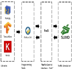
Pulai Perdana was selected as the case of study as it is one of the most congested traffic lights during the rush hours. Simulation of Urban Mobility (SUMO) was used to simulate the junction at Pulai Perdana as accurately as possible. Also, Python was utilized to interface with the simulation software and to deploy deep reinforcement learning to actuate the traffic signals. In Python, the deep learning library Keras was used to allow the algorithm to learn from its actions. Figure 1 demonstrate an overview of how the software interacts with each other to perform the simulation.
Figure 1 Simulation Software Architecture
Problem Definition
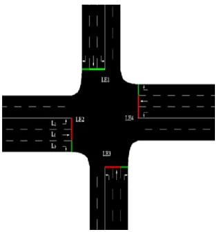
Perdana and LE4 shows traffic coming from Jalan Teratai. Each road was simulated to have 3 lanes in the signal side and 2 lanes on the other side as shown in Figure 2. A traffic video was taken for each road and fed into the Open CV algorithm by Özlü (2017) to count the number of cars passing through the junction during the rush hours. the traffic data obtained for an hour at the junction is shown in table 1.
Figure 2 Simulated Junction
Table 1: Traffic Information at Pulai Perdana Intersection
Junction Number of cars per hour
Green Signal Duration(s)
LE1 1076 100
LE2 796 38
LE3 1345 79
LE4 581 38
Vehicle Arrival Process
The traffic conditions are simulated based on Mathew (2014), which shows the method of simulating traffic flow through the use of random variates that follows the Poisson distribution to generate vehicles that arrives in a given time interval so that it follows a typical vehicle arrival process. In the SUMO simulation software, the traffic information is read from the route.xml file.
The Illustration of Vehicles arriving modelling is shown in figure 3.
Figure 3 Illustration of Vehicles arriving modelling
𝑝 𝑥 =𝜇𝑥𝑒−𝜇
𝑥! # 1
The Poisson distribution is commonly used to describe a random arrival process. Equation (1) is the probability of the density function.
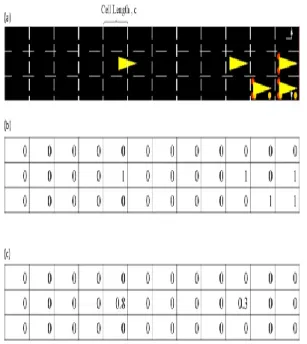
States
Figure 4: (a) Example of simulated traffic (b) with corresponding Boolean (c) and real-valued velocity vectors
Convolutional Neural Network
After observing the states, the agent was able to take an action based on what it “sees”. The process of seeing involves the use of a Convolutional Neural Network that allows extraction of important features from the state matrices.
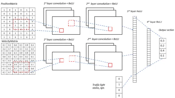
The input states or the agent’s observed states are positionMatrix, VelocityMatrix and lgts which are shown in figure 5. The first layer of convolution has 16 filters of 4x4 with stride of 2 and it uses ReLU (Rectified Linear Units) as the activation function. The second layer has 32 filters of size 2x2 with a stride of 1 and uses ReLU. The 3rd and 4th layers are fully connected layers with a size of 128 and 64 respectively. The final layer is then a layer with a linear output that outputs the Q value that corresponds to every possible action, this process is shown in figure 6.
positionMatrix = 𝑃0
𝑃1
𝑃2
𝑃3
,velocityMatrix = 𝑆0
𝑆1
𝑆2
𝑆3
,
lghts = 𝐿0
𝐿1
𝐿2
𝐿3
Figure 5: State matrices
Action
When the green light interval ended, the current time step t ended and a new time step began. The agent then proceeded to observe a new time step and chose the next action. The same actions might be chosen across time steps, causing the green light interval to run again for another 10 seconds. However, if the action selected was different from the previous action, such as changing the traffic signals. The yellow lights actuated for 3 seconds before actuating the green light. Since the agent’s goal was to reduce the overall waiting time, the agent needed to find an action policy that maximizes the following cumulative future rewards. After observing a given state, the agent decided to take an action based on an action policy π. The Traffic light phases for simulated lanes are shown in table 2.
Rewards
One of the biggest differentiators between reinforcement learning and other learning algorithms is the rewards. Rewards functions as a feedback system to allow the model to access its performance based on its previous actions. Since the main goal was to see if the model can increase the efficiency of the traffic light control system, the main parameters that can best reflect was the vehicle waiting time efficiency. Thus, we defined rewards as the difference in cumulative waiting time between active and number of vehicles previously in the inactive traffic, where r1 is the cumulative number of vehicles at a given active lane edge and r2 is the cumulative waiting time of idle vehicles waiting at the inactive lane edge.
The reward was then calculated after the agent finished its action step, which in this case, the reward was calculated after the 10 second period of actuation of the green light. Then the reward was reset to zero once the traffic agent changed the phase and restarted once again.
Agent Hyperparameters
The greedy epsilon algorithm was deployed, where the value of ε was 1.0 in the beginning to assume explorative behaviors, however, the value of epsilon started to decay at a rate of 99.5% every single time the states were observed until it
reached the minimum value of 0.01, where the agent started to change from taking explorative actions to exploitative one. The discount factor for future rewards was set at 0.95. The optimizer selected was then the Root Mean Squared Prop (RMSProp) algorithm, which used a moving average of squared gradients to normalize the gradient by itself, the algorithm was a stochastic technique for mini-batch learning. The learning rate for the RMSProp algorithm was set at 0.0002 for optimal results. The capacity of replay memory was also set at 200 to minimize memory usage.
Figure 6: Convolutional neural network approximating the Q values
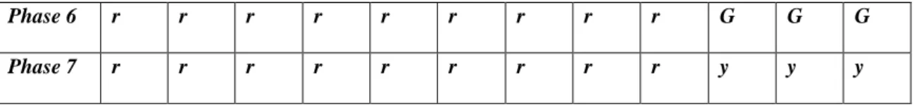
Table 2: Traffic light phases for simulated lanes.
LE1 LE2 LE3 LE4
L0 L1 L2 L0 L1 L2 L0 L1 L2 L0 L1 L2
Phase 0 G G G r r r r r r r r r
Phase 1 y y y r r r r r r r r r
Phase 2 r r r G G G r r r r r r
Phase 3 r r r y y y r r r r r r
Phase 4 r r r r r r G G G r r r
Phase 6 r r r r r r r r r G G G
Phase 7 r r r r r r r r r y y y
Agent Training
The agent was trained for 2000 episodes, each episode corresponds to 1 hour. We first initialized the neural network with random weights. At the start of each time step, the agent observed the current time step St and the input was fed into the neural network and performs an action At that would provide the highest cumulative future reward. The agent then received a reward Rt and proceeded to obtain the next step St+1 in the environment. These information (St, At, Rt, St+1) were stored as experiences in its memory. As the memory was limited in size, the oldest data was deleted when the memory was full. The DNN was then trained by extracting training examples from the memory. This was known as experience replay. The agent then proceeded to learn features \theta,
by training the DNN network to minimize the following Mean Squared Error (MSE) in (3).
𝑀𝑆𝐸 𝜃 =1
𝑚 𝑅𝑡+ 𝛾 max𝑎′ 𝑄(𝑆𝑡+1 , 𝑎′ ; 𝜃′) − 𝑄 𝑆𝑡𝐴𝑡; 𝜃 2 𝑚
𝑡=1
3
Since m was the size of the input data set, which in our case was very large, it would be very computationally expensive to calculate. Hence, we would use the stochastic gradient descent algorithm RMSProp with a minibatch of 32.
Figure 7: Graph of Cumulative Waiting Time Against Epoch 100000
150000 200000 250000 300000 350000 400000 450000 500000
0 200 400 600 800 1000 1200 1400 1600 1800 2000
Cumulati
ve
wai
ting ti
me
(s)
Epoch
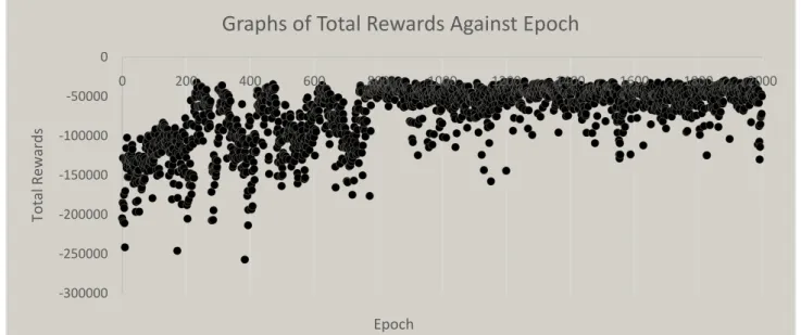
Figure 8: Graph of Total Rewards Time Against Epoch
RESULTS
&
DISCUSSION
By examining our simulation data shown in figure 7 & 8, we were able to show that the algorithm was indeed in the right path in learning a good action selection policy that effectively reduced the cumulative vehicle waiting time at the traffic lights. Our algorithm’s results started to converge midway through the episodes and became more stable.
During the training, the minimum cumulative waiting time achieved was 115882 seconds. The average value of the cumulative waiting time of all vehicles at the junction was 203221 second. At 200 episodes, we saw the waiting time of vehicles at the junction gradually reducing as the agent found suitable action policies that allowed it to make better decisions. The spikes in the graphs shows that the explorative nature of the agent allows it to try out different actions, not necessarily resulting in reduction in waiting time but crucial for exploring different actions that may give positive results. At 800 episodes, we saw the results started to converge and the waiting time started to stabilize from this episode onwards. The
stabilizing mechanisms such as the experience replay was proven to be effective in stabilizing the action selection policy.
After running the training for 2000 episode, the agent learnt a good action selection policy and managed to reduce the cumulative waiting time. The agent was then used to run the simulation once again using several carrying traffic conditions and compared to the fixed time algorithm. The agent was tested on high traffic conditions, high traffic conditions with traffic skewed to another direction, medium traffic conditions and low traffic conditions in comparison with the fixed time algorithm to evaluate its performance improvement as compared to the fixed time algorithm.
The skewed traffic was simulated by adjusting the heavy traffic to lanes LE2 and LE4 instead of LE1 and LE3. The medium traffic and low traffic were assumed at 50% and 20% of the high traffic volume. Table 3 shows the simulated result using the final weights of the algorithm after 2000 episodes of training.
-300000 -250000 -200000 -150000 -100000 -50000 0
0 200 400 600 800 1000 1200 1400 1600 1800 2000
Total
Rewar
ds
Epoch
Table 3 Cumulative Waiting Time for Different Algorithms and Traffic Heaviness. Traffic Heaviness Number of cars in
one hour in given lane
Cumulative Waiting Time (s)
LE1 LE2 LE3 LE4 Agent Fixed time algorithm
High 1076 796 1345 581 213696 405587
High (skewed traffic)
581 1076 796 1345 214522 704820
Medium 538 398 673 291 48592 153566
Low 215 159 269 116 18206 59549
Based on the results shown in table 3, it is clear that the agent outperforms the fixed time algorithm in every type of traffic heaviness, where in high traffic conditions, high traffic conditions with skewed traffic, medium traffic conditions and low traffic conditions, there is a 47.31 %, 69.56% ,68.36 % and 69.43 % reduction in waiting time respectively. The fixed time algorithm worked well at high traffic conditions, however, as the signal timing was set to meet the demand of the junction, it’s performance greatly reduced when the traffic was skewed to another direction. Although the number of cars passing through the intersection was the same, the fixed time algorithm could not handle the change in direction of the traffic heaviness as it was preset to a certain timing algorithm. The agent on the other hand was adaptive to traffic and was able to keep the cumulative waiting time at a constant value of 213696s and 214522s. This showed that the agent was adaptive and could execute a traffic control policy to solve the current traffic conditions. When the traffic heaviness was reduced to 50 % and 20 % respectively, we could see that the performance of the agent was 68.36% and 69.43% better than the fixed time algorithm. The performance was also better as compared to the high traffic conditions. The fixed time algorithm was not suited to adapt to the everchanging traffic heaviness, especially at lower traffic conditions.
CONCLUSION
In this paper, we proposed to solve the traffic light control problem at the Pulai Perdana intersection using a deep reinforcement learning model. This research study was a success with all objectives
achieved. The research started with the notion that artificial intelligence could one day be used as an agent to manage a traffic intersection by controlling the traffic lights. It was proven in this experiment that a deep reinforcement learning model is able to reduce the cumulative waiting time of all the vehicles at a given traffic junction as compared to a fixed time algorithm-based traffic management system at Pulai Perdana by 47.31%.
ACKNOWLEDGEMENT
The authors are grateful to the UniversitiTeknologi Malaysia for providing the funding for this study under the Research University Grant (RUG) with a vot number 03G98. The financial support is managed by the Research Management Centre (RMC) UniversitiTeknologi Malaysia.
REFERENCES
[1] Gao, J., Shen, Y., Liu, J., Ito, M., &Shiratori, N. (2017). Adaptive Traffic Signal Control: Deep Reinforcement Learning Algorithm with Experience Replay and Target Network. arXiv preprint arXiv:1705.02755.
[2] Genders, W., &Razavi, S. (2016). Using a deep reinforcement learning agent for traffic signal control. arXiv preprint arXiv:1611.01142.
[3] Li, L., Lv, Y., & Wang, F.-Y. (2016). Traffic signal timing via deep reinforcement learning. IEEE/CAA Journal of AutomaticaSinica, 3(3), 247-254. [4] Liang, X., Du, X., Wang, G., & Han, Z. (2018). Deep
reinforcement learning for traffic light control in vehicular networks. arXiv preprint arXiv:1803.11115.
[6] Özlü, A. (2017). Vehicle Detection, Tracking and Counting.
https://github.com/ahmetozlu/vehicle_counting