Published online December 30, 2012 (http://www.sciencepublishinggroup.com/j/ajnc) doi: 10.11648/j.ajnc.20120101.11
Matrix inversion algorithm: applications in high speed
MIMO LTE receiver
Md. Abdul Latif Sarker
1,2,*, Moon Ho Lee
1,21Dept. Of Electronic Engineer, Jeonju City, Republic of Korea 2Chonbuk National University, Jeonju City, Republic of Korea
Email address:
[email protected] (Md. Abdul Latif Sarker), [email protected] (M. Ho Lee)
To cite this article:
Md. Abdul Latif Sarker, Moon Ho Lee. Matrix Inversion Algorithm: Applications in High Speed MIMO LTE Receiver. American Journal of Networks and Communications. Vol. 1, No. 1, 2012, pp. 1-6. doi: 10.11648/j.ajnc.20120101.11
Abstract:
Matrix inversion algorithm acting an important role in MIMO wireless communication.In this paper, we pre-senta matrix inversion algorithm and it’s applications in the high speed MIMO LTE receiver which is based on floating point DSP. Matrix operations are the most costly computational module within MIMO receivers but a matrix inversion algorithm is very easy to compute and significantly reduce the computational module cost. We will demonstrate the MIMO LTE appli-cations for reducing the module cost by square matrix inversion algorithms.Keywords:
System Model;MIMO-LTE, Matrix Inversion Algorithm; Polar Decomposition, Matrix Inversion; Floating Point DSP, Implementation1. Introduction
Multi Input Multi Output (MIMO) -Long Term Evolu-tion (LTE) is the one of the newest technologies in wireless communications to improve bandwidth utilization efficien-cy. The access mode of multi-user MIMO LTE using a popular digital scheme Orthogonal Frequency Division Multiple Access (OFDMA) for downlink and Sub-Carrier Frequency Division Multiple Access (SC-FDMA) for up-link which provides high data rate in wireless environments. Multiple access channels are achieved in OFDMA by as-signing narrow sub-bands, each narrow sub-band has a flat frequency response and frequency selective channel is converted into a lot of flat-fading sub-channels. This can achieve a higher MIMO spectral efficiency averaging in-terferences from neighbouring cells and less affected to various kinds of impulse noise. The floating point DSP’s have better precision, higher dynamic range, and a smaller development cycle. These features result in reduced receiv-er complexity. This papreceiv-er is organized as follows: In sec-tion 2, 3 and 4, we have described system model, matrix inversion algorithms and polar decomposition with matrix inversion respectively. The implementation and simulation results are illustrated in Section 5. Finally, conclusions are presented in Section 6.
2. System Model
Most of the detection or the equalization processneeds to invert a matrix which is either the channel state information ( )W or a nonlinear function of it (function( )W ). If in-creasing the number of transmitter and receiver antennas is provide a higher data rate and the dimension of matrix function f w( ) increases, for more computations to invert the matrix in fewer times. In computing, floating point sys-tem represents real numbers which support a wide range of values. The numbers are in general represented to a fixed point or fixed numbers are of significant digits and scaled using an exponent. The base for the scaling is normally 2, 10, and 16. Symbolic form * e
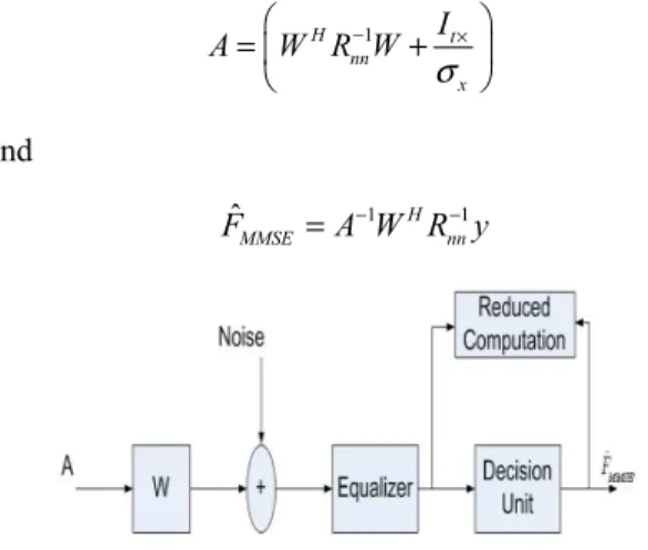
s b , where s is the value of the significant, b is the base, e is the exponent. The advantage of floating point over fixed point representation is that it can support a much wider range of values. The floating point format needs slightly more storage, if stored in the same space; floating point numbers achieve their greater range at the expense of precision. The speed of floating point opera-tions is an important measure of performance for computa-tion. For LTE application we have used MMSE equalization or detection algorithm. In Figure 1 shows the MMSE de-tection block diagram.
Let A is the 4x4 matrix for 4-steam MIMO-LTE and
ˆ
MMSE
1
H t
nn x I
A W R W
σ
− ×
= +
(1)
and
1 1
ˆ H
MMSE nn
F =A W R y− − (2)
Figure 1. Block diagram of MMSE detector.
3. Matrix Inversion Algorithms
For matrix inversion, the size of the matrix is larger than 2 2× in fixed- point implementation. The fixed-point algo-rithm has poor stability but floating-point work well and computation time requires fewer cycles like as cofactor, block-wise and systolic array method for matrix inversion operations as bellows:
3.1. Matrix Inversion Using Cofactors Algorithm
Let Abe the n n× matrix, the Mijis the determinant of
the sub-matrices of A and Cij is the cofactor ofaij, the
matrix of cofactor formed
11 12 1
21 22 2
1 2 ... ... ... n n
n n nn
C C C
C C C
A
C C C
=
⋮ ⋮ ⋱ ⋮ and
the cofactor ( 1)i j
ij ij
C = − + M , where th
i is the row, jththe column of the matrixA. The adjoint of Ais the transpose of the matrix of cofactors and it is denoted by adj A( ) . If
A is invertible matrix then 1 1 ( )
det( )
A adj A
A − =
, for a
MIMO LTE application we have used 4 4× matrix as an example, the inversion of a matrix Acan be written as [10], [11]:
11 12 13 14
21 22 23 24
1
31 32 33 34
41 42 43 44
1 1
( )
det( ) det( )
C C C C
C C C C
A adj A
C C C C
A A
C C C C
− = = (3)
To compute sub-matrices M12 where i=1 and j=2 which will be neededforC12. To compute the determinant of the matrix we get by removing the first row and second column. Here is that work
11 12 13 14
21 23 24
21 22 23 24
12 31 33 34
31 32 33 34
41 43 44
41 42 43 44
a a a a
a a a
a a a a
M a a a
a a a a
a a a
a a a a
⇒ ⇒
Now we can get the cofactor of the matrixA,
21 23 24
3 3
12 12 31 33 34
41 43 44
( 1) ( 1)
a a a
C M a a a
a a a
= − = −
. The determinant
of sub-matrices can be calculated from its diagonal values. For floating-point implementation, one division is used for computation of1 / det( )A .
3.2. Block-wise Matrix Inversion Algorithm
Matrices can be inverted block-wise by using Schur complement. For matrix inversion divides a square matrix into equal small matrices. Let 4x4 matrixes A, it is divided into four 2x2 sub-matrices and inverses by using the fol-lowing formula [8]:
P Q A
R S
=
(4)
whereP= ×m m,Q= ×m n,R= ×n m, S= ×n n ma-trix and Sis the invertible. The inversion each sub-matrices of matrix A as shown in Figure 5 and given by,
1 1
1
1 1 1
X P QY
A
Y RP Y
− − − − − − − = −
(5)
whereX=P−1+P QY RP−1 −1 −1 andY= −S RP Q−1 .
Figure 5. Block-wise matrix inversion algorithm.
The common parts of -1
P , 1
RP− and 1
1
1 p q 1 s q
A
r s ps qr r p
−
− = = −
− −
(6)
The matrix A has complex conjugate symmetric values of non-diagonal components for all targets sub-matrices in the MMSE detection and (ps−qr) becomes a real value in this case.
3.3. Systolic Array Process
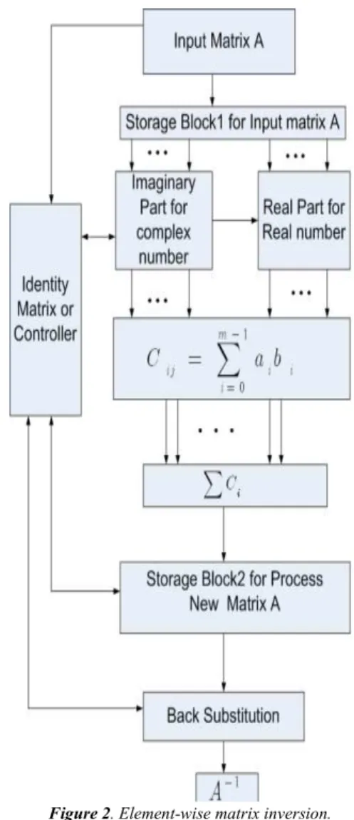
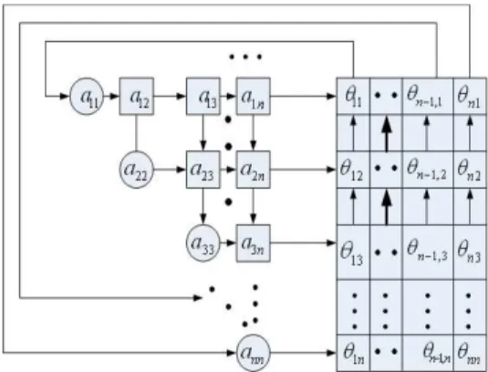
Systolic array is a computing communication processing which has some advantage like as synchrony, modularity and regularity, spatial and temporal locality, pipelining etc. For computation, it is a simple and regular design, network and balancing computation with input and output. The block diagram of the matrix inversion process and the complete multiplication of sub-matrices using a systolic array process in Figure 2 [2], [3], [6], Figure 3 and Figure 4 [6] the ele-ment-wise inversion algorithm for matrix triangulization and it is involves local communication between nodes which is suitable for hardware implementation. The triangle has two different blocks. One is real values block and another is imaginary values block. These two parts perform rotations on each element in input matrix as shown in Figure 2. Vector operation on imaginary inputs valued which means it nulli-fies the imaginary parts of a complex number and outputs the rotation angle to the real parts. Let A is the 4 4× input matrix and I is the identity matrix or the controller of the system as shown in Figure 2. Initial state the operation of input matrix inversion is stored in storage block1. After receiving the first value, imaginary block start processing it. Imaginary block does not have to wait for the first step to finish and these two states can be pipelined. The imaginary block performs vector zing on the values and sends the rotation angle to the real block. The output of the imaginary blocks enters the real blocks for more processing. After processing, all values are stored in storage block 2. The final output inverse of a matrixAis stored in storage block 2. The identity matrix I controls the flow of inputs and outputs to each imaginary & real block and storage blocks of the sys-tem. In Figure 4, the tri-array provides upward and rightward communication channels, as opposed to the downward and rightward ones provided in the first phase processing. In Figure 4, if
θ
= °45 andLet,
c o s 4 5 s in 4 5 1 1
s in 4 5 c o s 4 5 2 1
i U
i
° − ° −
= ° ° =
,
We can express by [11]:
1
1 1 e 0 1
1 1
1 0
2 2
i i
i
U U
i i e i
θ
θ
∆
− − ∆
= Λ
− −
(7)
whereΛis diagonal and phase shift matrices.
Figure 2. Element-wise matrix inversion.
Figure 4 .The Parameters of the rotation angles {θi j}emerge from the
right side and data buffer to store these parameters with the top -row connected to the diagonal processing elements of the tri-array.
4. Polar Decomposition with Matrix
Inversion
If A is non-singular squaren n× matrices, A∈ℂn n× this
algorithm computes the polar decomposition,
A=QU =VQ (8)
where Q is the orthogonal matrix, U is the symmetric positive definite matrix and right stretches. The forward (upper) operation of the polar decomposition inA,
2 *
U =A A (9)
where
( )
⋅* denotes transpose conjugate. Similarly the reverse (lower) case,A VQ= (10)
whereV2 =AA*whereV is symmetric and left stretches. The Principal rotation matrix as given by
1 1
Q=U A− =AV− (11)
whereU=Q A* =Q VQ*
andV =AQ* =QUQ*
. If A is nonsingular non-square (m n× ) matrices and A∈ℂm n× this
can first calculate QR decomposition [7],
A=QR (12)
whereQ∈ℂm n× has orthogonal column, Ris upper
tri-angular and nonsingular. The polar decomposition of Ais given in term of that of Rby
( R R) ( R) R
A=QR=Q U V = QU V =UV (13)
Let Sub-matrices i j
a b
M
c d
=
of matrixA, then a
factor that makes unit columns vectors
d e t( )
ij ij
d c
Q M s ig n M
b a
−
= + −
.The Polar decomposition
factor Q is the closest possible to matrixMij, with norm
measured using Frobeniusnorm Q−Mij F2 . We can
ex-press Mij F2 as the diagonal sum and trace of M M* us-ing a symmetric Lagrange multiplier matrixr.
[( ) (T ) ( T ) ]
ij ij
trace Q M− Q M− + Q Q−I r (14)
We can differentiate with respect to Q and express by
( )
ij
M =Q I+ =r QU (15)
where (I+r) is the forward polar symmetric positive upper triangular and right stretches matrix. Similarly we can write,
( )
ij
M = −I r Q=VQ (16)
where (I−r) is the reverse polar symmetric lower tri-angular and left stretches matrix.
This factorization is the polar decomposition ofMij. We
can write
1 * 1
(MU−) (MU−)=I (17)
whereQ QT =I and symmetric inverse is given by
1 * 1
2 *
U M MU I
U M M
− − =
∴ = (18)
Similarly we can write by equation (17)
2 *
V =MM (19)
From equation (2) matrix inversion of A to get an MMSE solution using lower and upper triangular, forward polar and reverse polar operations as below:
1
ˆ ˆ
MMSE
F =A y− (20)
where ˆ H 1
nn y=W R y− . For lower triangular case:
2ˆ *ˆ
ˆ MMSE MMSE
y=V F =MM F (21)
and for upper triangular case:
2 *
ˆ ˆ
ˆ MMSE MMSE
y=F U =F M M (22)
5. Implementation and Simulation
Re-sults
Matrix Ais a 4 4× matrix of complex, floating point values and output is the inverse matrix. In Figure 5, the
sub-matrix 1 1
P QY− −
− can be computed from the hermitian
transpose of 1 1
Y RP− −
− . Matrix Ahas four 2 2× sub-matrix
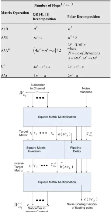
arithmetic units. These units are to be implemented using pipeline circuit in Figure 5 and Figure 6.The number of computation depends on the number antennas Land the cost of MMSE equalizer for 4 4× matrix inversion as fol-lows [4]:
3 2
10 5
flops
f = L + L +L(23)
The noise covariance matrix Rnn1
−
in equation (1) is a diagonal matrix and all diagonal elements are equal. We assume equal noise variance and additive white noise for all receive antennas. In Figure 6, the inverse channel matrix:
(
)
11 2
k k k
H H
sc sc sc sc
W− = W W +σ I − W (24)
The target matrix k k 2
H sc sc sc
T =W W +σ Iand the output of
the equalizer:
1 1 1
ˆ ( ) ( ) ( ) ( )
k k k k k k k
H H
MMSE sc sc sc sc sc sc sc
F t =W− y t =T W− y t = A W− y t (25)
whereTsc1k A1
− = −
and sck is the number of sub-carrier
and t the number of step for MIMO receiver. The receiver
complexity O
{ }
( )
E L where L is the numberof receiver antennas and the processing elementsE. In Figure 6, the block floating scaling factors are settled to decrease the finite length errors in the 2 2× sub-matrix multiplication and inverse units. Complex floating point operations (flops) scaling for each scalar complex addition count one flop and each complex multiplication count three flops. For squarematrices n n
A∈ℂ× , n n
B∈ℂ× , n n
C∈ℂ× and complex vector
1
ˆ n
d∈ℂ× , the computational cost of the matrix operation, number of flops and useful vector counts between QR and polar decompositions are as shown in Table 1.Simulation results from the matrix inversion algorithms using polar decomposition, floating point operation (25) we tested as shown in Figure 7and Figure 8. The BER performance on without channel matrix inversion is compared to that of with channel matrix inversion algorithm for 4 4× case in which four receivers with the highest norm values are selected out of number of users has been shown in Figure 9.It can be mitigated noise enhancement very fast.
Figure 7. Matrix inversion using polar decomposition (matrix size 16x16).
Table 1. Compare to QR and Polar Decomposition.
Matrix Operation
Number of Flops(ff l o p s) QR [4], [1]
Decomposition Polar Decomposition
A+B n2 n2
A*B 3
2n / 3 n3/ 3
A*AH
(
4n3+ −n2 n)
/ 2( )
(
)
31 / 6
N− n
where
. .
N=no of iterations 1 2
* *
;
A=MM M =QA
C-1 3 2
4n +n +n 2n3+n2−n
A*a 2
4n −n 2
2n −n
Figure 6. Block diagram of transmission architecture.
Figure 8. 16x16 channel matrix inversion. 0.1
0.2 0.3
30
210
60
240
90
270 120
300 150
330
180 0
-0.500.5 -0.500.5 -0.500.5 -0.500.5 -0.500.5 -0.500.5 -0.500.5 -0.500.5 -0.500.5 -0.500.5 -0.500.5 -0.500.5 -0.500.5 -0.500.5 -0.500.5 0.250.250.25 -0.50
0.5 -0.50 0.5 -0.50 0.5 -0.50 0.5 -0.50 0.5 -0.50 0.5 -0.50 0.5 -0.50 0.5 -0.50 0.5 -0.50 0.5 -0.50 0.5 -0.50 0.5 -0.50 0.5 -0.50 0.5 -0.50 0.5 0.25 0.25 0.25
Figure 9. BER performance using matrix inversion algorith.
6. Conclusions
Matrix inversion is designed and implemented on various types of DSP’s like as Xilinx vertex 5 using cofactors, block- wise, systolic array and polar decomposition methods in floating point. All 32 bits are real and imaginary precision. One sign bit and 8 exponents bit. Word length
( )
l of 4 4× the matrixhas a floating-point C block-wise cycles1 ( ) k
sc
l+A y− t and floating point cofactor 1 ( )
k
sc l+A y− t
and block-wise methods save about 3 to 4 times the fixed-point polar decomposition based inversion in terms of cycle counts. Polar decomposition factor (8) QUwhich are unique, independent coordinates, both efficient and easy to compute. So our proposed method increasing the matrix inversion processor clock speed and reduces the receiver computational module cost.
Acknowledgements
This work was supported by World Class Universi-ty-R32-2010-000-20014-0, the NRF, BSRP-2010-0020942, NRF, BK21 and MEST-2012-002521, NRF, Republic of Korea.
References
[1] M. Myllyla, J. Hintikka, J. Cavallaro, M.Juntti, M. Limingoja, and A. Byman, “ Complexity Analysis of MMSE Detector Architecture for MIMO-OFDM System,” in Proceedings of the 2005 Asilomar Conference, Pacific Grove, CA, Oct 30-Nov 2 2005.
[2] “www.Altera.com”, “www.Xilinx.com”.
[3] H. K. W. M Gentleman, “MatrixTriangularization by Sys-tolic Arrays”, Real-Time Signal Processing, vol.298, pp.19-26, 1981.
[4] Mohamed Chouayakh, AndressKnopp, and Berthold Lankl, “Low Complexity Two Stage Detection Scheme for MIMO Systems” IEEE Information Theory for Wireless Network, 1-4244-1200-5/07/2007.
[5] Di Wu. Johan Eilert and Dake Liu, Dandan Wang, Naofal Al-Dhahir and HlaingMinn, “Fast Complex Valued Matrix Inversion for Multi-User STBC MIMO Decoding” VLSI, 2007, ISVLSI ’07, IEEE Computer Society Annual Sympo-sium, pp.325-330, March 2007.
[6] MarjanKarkooti, Josep R. Cavallaro, Chris Dick, “FPGA Implementation of Matrix Inversion Using QRD-RLS Algo-rithm,” 1-4244-0132-1/2005 IEEE.
[7] LuoJianwen, Jong ChingChuen, “Matrix Inversion on Re-configurable Hardware Using Binary –Coded Z-Path COR-DIC,” APCCAS 2006.
[8] Shodai Yokoyama, Kazuya Matsumoto, and Stanislar G. Sedukhin,” Matrix Inversion on the Cell/B.E. Process,” 11th IEEE International Conference on High Performance Com-puting and Communication, 2009.
[9] Moon Ho Lee,SundarRajan, J.Y. Park, “A Generalized Re-verse Jacket Transform,” IEEE Transactions on Circuit Sys-tems-II: Analog and Digital Signal Processing, Vol.48 No.7, July 2001.
[10] Moon Ho Lee, “A New Reverse Jacket Transform and Its Fast Algoritham,” IEEE Transactions on Circuit Systems-II: Analog and Digital Signal Processing, Vol.47 No.1, July 2000.
0 2 4 6 8 10 12 14 16 18 20
10-3 10-2 10-1 100