*Correspondence to Author:
Yaya Sudarya Triana
Information Systems Department, Information System, Universitas Mercu Buana Jakarta, Indonesia
How to cite this article:
Yaya Sudarya Triana.Monte Carlo Simulation for Modified Paramet-ric Of Sample Selection Models Through Fuzzy Approach.American Journal of Basic and Applied Sci-ences, 2018, 1:6
eSciPub LLC, Houston, TX USA. Website: http://escipub.com/
Yaya Sudarya Triana , AJBAS, 2018 1:6
American Journal of Basic and Applied Sciences
(DOI:10.28933/AJBAS)
Research Article AJBAS (2018) 1:6
Monte Carlo Simulation for Modified Parametric Of Sample
Selection Models Through Fuzzy Approach
The sample selection model is a combination of the regression and probit models. The models are usually estimated by Heck-man’s two-step estimator. However, HeckHeck-man’s two-step estima-tor often performs poorly. In the context of parametric methods, the sample selection model is studied. The best approach is to take advantage of the tools provided by the theory of fuzzy sets.
It appears very suitable for modeling vague concepts. It is diffi -cult to determine some of the criteria and arrive at a quantitative value. Fuzzy sets theory and its properties through the concept of fuzzy number. The fuzzy function used for solving uncertain of a parametric sample selection model. Estimates from the fuzzy are used to calculate some of equation of the sample selection model. Finally, estimates of the Mean, Root Mean Square Error (RMSE) and the other estimators can be obtained by Heckman two-step estimator through iteration from some parameters and some of values.
Keywords: Fuzzy, Heckman’s, Monte Carlo, Sample selection model, Simulation
Yaya Sudarya Triana
Information Systems Department Information System, Universitas Mercu Buana Jakarta, Indonesia
ABSTRACT
I. INTRODUCTION
The sample selection was developed by [1]. Sample selection
is widely used in various fields of economics. An early discussion of the problem of self-selectivity was that of [2], who discussed the problem of individuals selecting between hunting and fishing, based on their comparative advantage. The observed distribution of incomes of hunters and fishermen was defined by these choices [3]. The self-selectivity model that focused on selectivity bias was discussed by [4]. [5] introduced a two-step selection model, known as the Heckman two-step sample selection model. The sample selection bias problem in the context of decision by women to participate in the labour force is discussed by [4], [6], [1], [7], [8], [9] and [10].
II. PARAMETRIC SAMPLE SELECTION MODEL [11] has proposed the parametric sample selection model as follows :
The variables and are unobserved,
whereas yi is observed. and are dependent variables, xi and wi are vectors of independent variables, α and β are unknown parameter vectors, ui and vi are error terms. In Equation (1), there are error terms (u, v) which are usually correlated, so that the regression of y on x will not a give consistent estimates of β0 and β1. The approach of the error terms (ui, vi) are assumed to follow a bivariate normal distribution. It is commonly assumed that ui and
vi have a bivariate normal distribution :
According to [12] and [13], there are two parts in Equation (1). The first part is participation equation (a binary decision equation). The second part is the wage equation (outcome equation or selection part). Independent variable xi usually contain at least one variable which does not appear in variable wi. The outcome equation describes the relationship between the dependent variable yi and independent variable xi, whereas in the selection equation describes the relationship between the dependent variable di and the independent variable wi.
III. ALPHA-CUT OF FUZZY NUMBER
Alpha cuts are simply threshold levels that convert a fuzzy set
into a crisp set. The process of converting a fuzzy set to a crisp one is called defuzzification. An alpha-cut A of a fuzzy number A is defined as the set {x R | A(x) }. A is completely determined by the collection ( )0,1]. An
alpha cut is the behaviour sensitivity of the system to the behavior under observation. At some point, as the information value diminishes, one no longer wants to be "bothered" by the data. In many systems, due to the inherent limitations of the mechanisms of observation, the information becomes suspect below a certain level of reliability.
simple since only two simulations will be enough for each α-level (one for each boundary). Otherwise, optimization routines have to be carried out to determine the minimum and maximum values of the output for each α-level. Figure 1 shows an illustration of the alpha-cut of triangular fuzzy number.
From Figure 1, the confidence fuzzy interval defined by different value of alpha cut. For example : α(0.4) and (0.8), then their confidence fuzzy interval are [BL, BU] and [CL, CU]. This relationship denoted by (α(0.4), [BL, BU]), and (α(0.8), [CL, CU]) with [BL, BU] ≥ [CL, CU]. IV. THE MODEL
In this section the model of participant, non-participant, and combination of participant and non-participant are discussed. The model is written as follows :
where di is a selection equation of the first stage. The values of di are 0 and 1 which is di = 1 for participant and di = 0 for nonparticipant. yi is dependent variable of the outcome equation. In the Equation (2) is derived into two, ie y0 and y1. y0 is refered to the outcome of the Equation (2) is non-participant, whereas y1 for participant. xi is independent variable. The details about the
equation of y1 and y0 are as follows :
where u0i and u1i are error terms. The outcome equation for non-participant and participant in Equation (2), can be summarized as follows :
hence, the combination of both non-participant and participant, will generate the equation, as follows :
V. MONTE CARLO SIMULATION OF PARAMETRIC SAMPLE SELECTION MODEL
The purpose of the Monte Carlo simulation is used to calculate the values of the sample selection model [14]. The fuzzy model for Monte Carlo simulation is as follows :
The following items are considered in the Monte Carlo study: - The effect of the correlation of ~xi and w~i
- The effect of the correlation of ~ui and ~vi
~s1i and ~s2i are independent and identically distributed (i.i.d.) random variables distributed uniformly on (0,20]. The values of the
exogenous variables, ~xi and w~i are as
follows :
~s1i and ~s2i are random uniform variables with mean = 0 and variance = 20. π is the correlation
coefficient of ~xi and w
~
0.9 are considered. The fuzzy error terms{(~ui ,~vi )} are jointly normal and
determined as follows:
are normal random variables with mean =
0 and variance = 1 are i.i.d. normal random
variables with mean = 0 and variance = 100. and are independently distributed
is the correlation coefficient of ~ui and ~vi with values of ρ0 = 0.0, 0.5, and 0.9 considered. The
error terms are calculated twice, which is for the classical error terms as well as the fuzzy error terms. ρ from [-0.99, 0.99] with interval 0.01. The true values of the parameters are β0 = -10.0, β1 = 1.0, α0 = -1.0, and α1 = 0.1,
Our hypothesis is H0: β1 = 0 against H1: β1 ≠ 0. If the hypothesis testing fails to reject H0, meaning that the model does not reflect our data. The sample sizes n=100, 200, and 400 are considered with 1000 replications on each sample size.
True value is the actual variation that would be measured. In this case, so that the expected results are similar to the entered value, the true value for β0 and β1 are -10.0 and 1.0 is expected to result from these estimates and values. The chosen sample size, n = 100, 200 and 400 are only example values, this value is expected to meet the minimum value that should be taken, should we take another value, e.g. 101, 213, 379, etc. The larger the sample size and replication, the better. So as the normal random value is generated, this value is exemplified by a normal distribution (0.1) which means normal standards of raw materials, normal distribution (0.100) and the uniform normal distribution (0.20). This simulation will be measured in the range and value, so hopefully the results will be
in the range of the accepted values.
VI. RESULT
The calculation of Monte Carlo simulation from Table 1 to
Table 5 using fuzzy α-cut 0.2, 0.4, 0.5, 0.6, 0.8, and 1.0. The effect of correlation can be viewed from the fuzzy exogenous variables between w~ and ~x and the effect of correlation of fuzzy error terms between ~u and ~v , and the effects of comparison among several different sample sizes are n = 100, n = 200, and n = 400, shown in the table on the columns 1, 2 and 3, while columns 4, 5, 6 and 7, 8, 9 show Mean, SD and RMSE of parameter β0 and β1, where SD is standard deviation and RMSE is root mean square errors.
Result is shown from Table 1 to Table 5 are the Mean, SD, RMSE with n=100, 200 and 400 for parameters of β0, β1. From this table, represented the α-cuts of triangular fuzzy number with a value of 0.2, 0.4, 0.5, 0.6, and 0.8. The first column shows the parameter of phi with values 0.0, 0.5, 0.9, while the second column shows the parameter of rho with a value of 0.0, 0.5, 0.9.
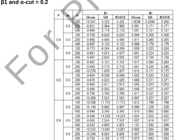
Table 1 display that the mean of parameters of β0 and β1 showed about the consistency information of the parameter estimator that approaches the true values, while the SD and RMSE provide information about the level of efficiency for the parameters in the estimation. Sample size n = 100, n = 200 and n = 400 provides the information that the larger the sample size, the smaller the values of SD and RMSE, it means that more efficient and accurate the estimator, if there is no relationship between fuzzy error term.
the values of SD = 2.964, RMSE = 2.969 of parameter of β0 and the values of SD = 0.171, RMSE = 0.171 of parameter of β1, while for the sample size n = 400, the values of mean of parameters β0 = -9.969 and β1 = 1.001, the values of SD = 2.116, RMSE = 2.116 of parameter of β0 and the values of SD = 0.121, RMSE = 0.121 of parameter of β1.
Result of Mean, SD, RMSE of FMPSSM with n=400 for β0, β1 and α-cut = 0.2 From Table 1, it can be shown that for the α-cut = 0.2, with sample size n = 100, where values of ρ0 and π are 0 (meaning that there is no relationship between ρ and π), so the value becomes small of SD and RMSE for parameter of β0, the values of SD = 4.325, RMSE = 4.325 and for parameter of β1, the values of SD = 0.260, RMSE = 0.260. When the sample size increases and become n = 200, SD and RMSE values for the parameters β0 and β1 decreases, i.e. for value of SD = 2.964, RMSE = 2.969 of parameter β0, and the value of SD = 0.171, RMSE = 0.171 of the parameter β1. When the sample size increases again for n = 400, SD and RMSE values for the parameters of
β0 and β1 is smaller again, that is the values of SD = 2.116, RMSE = 2.116 for parameter of β0 and the values of SD = 0.121, RMSE = 0.121 for parameter of β1. While ρ0 increases to moderate values of 0.5 (moderate correlation between fuzzy error term), then the values of SD and RMSE becomes larger than when the value of rho = 0 (no error relationship between fuzzy terms).
Increase in value of ρ0 as shown in Table 1 indicates that the greater correlation of fuzzy error terms between ~u and ~v , the smaller the value of SD and RMSE. From the above table also illustrates, that when the value of ρ0 and π strong (ρ0 and π = 0.9), then the values of SD and RMSE increased, compared with the value of which no correlation of ρ0 and π are moderate. This shows that the occurrence of multicollinearity of fuzzy exogenous variables between
w~I and ~xi, but the value of this
multicollinearity will be corrected by sample size that continues to expand.
Table 1 : Mean, SD, RMSE of FMPSSM under normality assumption with n=100, 200, 400 for β0, β1 and α-cut = 0.2
Table 1 display that the mean of parameters of β0 and β1 showed about the consistency information of the parameter estimator that approaches the true values, while the SD and RMSE provide information about the level of efficiency for the parameters in the estimation. Sample size n = 100, n = 200 and n = 400 provides the information that the larger the sample size, the smaller the values of SD and RMSE, it means that more efficient and accurate the estimator, if there is no relationship between fuzzy error term.
For example in Table 6.1, for the sample size n = 100, the values of mean of parameters β0 = -10.0969 and β1 = 0.9967, the values of SD = 4.6709, RMSE = 4.6719 of parameter of β0 and the values of SD = 0.2530, RMSE = 0.2530 of parameter of β1, for the sample size n = 200, the values of mean of parameters β0 = -9.9669 and β1 = 0.9984, the values of SD = 3.0880, RMSE = 3.0882 of parameter of β0 and the values of SD = 0.1737, RMSE = 0.1737 of parameter of β1, while for the sample size n = 400, the values of mean of parameters β0 = -9.9701 and β1 = 1.0020, the values of SD = 2.1179, RMSE = 2.1182 of parameter of β0 and the values of SD
= 0.1249, RMSE = 0.1249 of parameter of β1. From Table 1, it can be shown that for the α-cut = 0.2, with sample size n = 100, where values of ρ0 and π are 0 (meaning that there is no relationship between ρ and π), so the value becomes small of SD and RMSE for parameter of β0, the values of SD = 4.6709, RMSE = 4.6719 and for parameter of β1, the values of SD = 0.2530, RMSE = 0.2530. When the sample size increases and become n = 200, SD and RMSE values for the parameters β0 and β1 decreases, i.e. for value of SD = 3.0880, RMSE = 3.0882 of parameter β0, and the value of SD = 0.1737, RMSE = 0.1737 of the parameter β1. When the sample size increases again for n = 400, SD and RMSE values for the parameters of β0 and β1 is smaller again, that is the values of SD = 2.1179, RMSE = 2.1182 for parameter of β0 and the values of SD = 0.1249, RMSE = 0.1249 for parameter of β1. While ρ0 increases to moderate values of 0.5 (moderate correlation between fuzzy error term), then the values of SD and RMSE becomes larger than when the value of rho = 0 (no error relationship between fuzzy terms).
Table 2 : Mean, SD, RMSE of FMPSSM under normality assumption with n=100, 200, 400 for β0, β1 and α-cut = 0.4
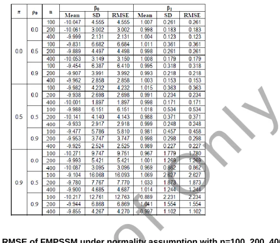
Table 3 : Mean, SD, RMSE of FMPSSM under normality assumption with n=100, 200, 400 for β0, β1 and α-cut = 0.5
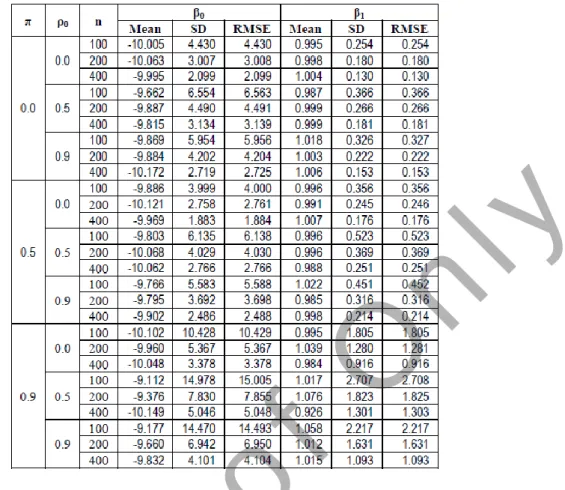
Table 4 : Mean, SD, RMSE of FMPSSM under normality assumption with n=100, 200, 400 for β0, β1 and α-cut = 0.6
Table 5 : Mean, SD, RMSE of FMPSSM under normality assumption with n=100, 200, 400 for β0, β1 and α-cut = 0.8
Table 5 : Mean, SD, RMSE of FMPSSM under normality assumption with n=100, 200, 400 for β0, β1 and α-cut =1.0
The consistency for FMPSSM and FMSPSSM has been discussed. The effect of the
correlation of variables
~xi and w~i , then the effect of the correlation of error terms ~ui and ~vi
are then observed. The FMSPSSM has used the bandwidth by the Powell estimator. The effects of bandwidth changes are studied and researched, and later observed whether it is consistent or not.
Table 6.1 to Table 6.5 are calculation of FMPSSM for Mean, SD, RMSE under normality assumption, Table 6.6 to Table 6.10 are calculation of FMPSSM for Mean, SD, RMSE under non-normality assumption. The values of SD and RMSE
decreased with increased sample size, and also decreases with increasing values of α-cut. The values of SDn100 > SDn200 > SDn400 and the values of RMSEn100 > RMSEn200 > RMSEn400. Table 6.11 to Table 6.15 are the calculation of FMSPSSM for Mean, SD, RMSE. From the tables it appears that the values
of SD and RMSE decreased with an increasing sample size, the α-cut, and the bandwidth. The results obtained from Monte Carlo simulations for the previous study, suggesting that FPSSM is consistent and efficient, the same as the results obtained with FMPSSM.
V. CONCLUSION
To reduce the problem of uncertainty that exists in the
parametric sample selection models, then created a fuzzy approach. fuzzy concept that used for modified of the parametric sample selection models provides an alternative for the handle to the problem when the model involves the characteristic vagueness, uncertainty and ambiguity.
Result of the Parametric Sample Selection Models using a fuzzy approach shows that the larger the sample size, the smaller the values of SD and RMSE, it means that the more efficient
and accurate the estimator, then the greater the value of α-cut, the smaller the values of SD and RMSE, and the more efficient and accurate.
REFERENCES
1. Heckman, J.J., “Shadow price, market wages and labor supply”, Econometrics, 42, p. 679-694, 1974. 2. Roy, A. D. (1951). Some Thoughts on the
Distribution of Earnings. Oxford Economic Papers, 3. 135-146.
3. Maddala, G.S., “Limited-dependent and qualitative in econometrics”, Cambridge University Press. p. 257-289, 1983.
4. Gronau, R., “Wage comparisons: A selectivity bias”, Journal of Political Economy, 82, p. 1119-1143, 1974.
5. Heckman, J.J., “Sample selection as a specification error”, Econometrica, Vol.47, p.153-161, 1979.
6. Lewis, H.G., “Comments on selectivity biases in wage comparisons”, Journal of Political Economy, 82, p. 1145-1155, 1974.
7. Neumark, D. (1988). Employers’ Discriminatory Behavior and the Estimation of Wage Discrimination. Journal of Human Resource, 23,279-295.
8. Gerfin, M. (1996). Parametric and semi-parametric estimation of the binary response model of labour market participant. Journal of Applied Econometrics, 11, 321-339.
9. Vella, F., “Estimating models with sample selection bias: A survey”, Journal of Human Resource, Vol. 33, p. 127-169, 1998.
10. Christofides, L. N., Li, Q., Liu, Z., & Min, I. (2003). Recent two-stage sample selection procedure with an application to the gander wage gap. Journal of Business & Economic Statistics, 21 (3), 396-405.
11. Heckman, J.J., “The common structure of statistical models of truncation, sample selection, and limited dependent variables, and a simple estimation for such models.”, Annals of Economic and Social Measurement, 5, 475-492.
12. Schafgans, M. (1996). Semi-parametric estimation of a sample selection model: Estimation of the intercept, theory and applications.Unpublished Ph.D. Thesis. Yale University. New Haven. USA.
13. Martins, M. F. O. (2001). Parametric and semiparametric estimation of sample selection models: An empirical application to the female labour force in Portugal. Journal of Applied Econometrics, 16, 23-39.
14. Nawata, K., “Estimation of Sample Selection Bias Models by Maximum Likelihood Estimator and Heckman’s Two-Step estimator”, Econometrics Letters, 45, 33-40, 1994.