Vol. 11, No. 4, 2018, 893-910
ISSN 1307-5543 – www.ejpam.com Published by New York Business Global
Proximity between selfadjoint operators and between
their associated spectral measures
Alain Boudou1, Sylvie Viguier-Pla2,1,∗
1Equipe de Stat. et Proba., Institut de Math´ematiques, UMR5219, Universit´e Paul Sabatier, 118 Route de Narbonne, F-31062 Toulouse Cedex 9, France
2 LAMPS, Universit´e de Perpignan, 56 avenue Paul Alduy, F-66860 Perpignan Cedex, France
Abstract. We study how the proximity between two selfadjoint bounded operators can be ex-pressed as a proximity between the associated spectral measures. Between two operators, we use a classical distance. For projector-valued spectral measures, we introduce the notion of
α−equivalence, which is based on a partial order relation on the set of projectors. Assuming an hypothesis of commutativity, we show that the proximity between operators is equivalent with the proximity between the associated spectral measures. We develop the particular case where the operators are compact, and give some illustrations.
2010 Mathematics Subject Classifications: 60G57, 60G10, 60B15, 60H05
Key Words and Phrases: Random measures, Stationary processes, Convolution, Spectral mea-sures
1. Introduction
The question of the association of a spectral measure (s.m.) with an operator is a usefull technique, and often considered for the analysis of their properties ([4], [3]). Therefore, if P is an orthogonal projector, andλa real, thenA=λP is a selfadjoint bounded operator, which associated s.m. isE =δ0P⊥+δλP. Besides, the null operatorO is associated with
the s.m. ER=δ0I.
AskA−Ok=|λ|,Aand O are two selfadjoint operators as close as we want, as far as we can get |λ| as small as we want. Nevertheless, let us consider the proximity between their associated s.m.’s. For anyB of aσ−field defined onR, we have
E(B)− ER(B) =δ0(B)P⊥+δλ(B)P−δ0(B)P⊥−δ0(B)P =δλ(B)P −δ0(B)P.
So kE(B)− ER(B)k=|δλ(B)−δ0(B)|, which maximum is obviously equal to 1.
This shows that the proximity between two s.m.’s, evaluated by sup{kE(B)−ER(B)k;B∈ BR}, is not appropriate to be linked with the proximity between their associated operators.
∗
Corresponding author.
DOI: https://doi.org/10.29020/nybg.ejpam.v11i4.2552
Email addresses: [email protected](A. Boudou),[email protected](S. Viguier-Pla)
In [2], we have seen how the proximity between unitary operators could be equivalent with proximity between their associated s.m.’s.
In this paper, we develop tools for the study of the association between selfadjoint bounded operators and s.m.’s. Our study of proximity is placed in this context.
In order to fix notation, Section 2 is devoted to the recall of some notions, as random measure, spectral measure, space of the measurable applications of integrable square with respect to a random measure, and projector-valued spectral measure. We introduce in a third section the notion of α−equivalence, for α positive real, between two s.m.’s. This concept of proximity can be translated by proximity between two selfadjoint bounded operators, what we will develop in Section 4. The fift section will be dedicated to the case of the compact operators, which is frequently encountered in numerical applications. A numerical illustration is given in the last section.
2. Recalls
2.1. Orthogonal families of projectors
In this text,H,L(H) andP(H) are respectively aC−Hilbert space, the set of bounded endomorphisms ofH(which is a Banach space for the normkAkL= sup{kAxk;kxk= 1}),
and the set of the orthogonal projectors onH.
Let P1 and P2 be two elements of P(H), P1 is said to be “less or equal” to P2, what
we denote P1 P2, ifP1P2=P1.
This defines, on P(H), a partial order relation.
A family {Pn;n∈N}of elements ofP(H) is said to be orthogonal whenPn◦Pm = 0,
for any pair (n, m) of distinct elements of N. Then we can show that a) for anyX of H, the family{PnX;n∈N} is summable;
b) the application P :X ∈H 7→P
n∈NPnX ∈H is an element of P(H) which we name
the sum of the orthogonal family of orthogonal projectors {Pn;n ∈ N} and which we denote P
n∈NPn;
c) for anynof N, we have Pn◦P =Pn.
We emphasize the fact that an orthogonal family of orthogonal projectors can be not summable (as a family of elements of the Banach spaceL(H)).
The following first result, which can be easily proved, will be used in Section 3. Lemma 2.1.1. If {Dn;n ∈ N} and {Dn0;n ∈ N} are two orthogonal families of orthogonal projectors of respective sum D and D0 such that Dn D0n, for any n of N, thenDD0.
2.2. Random measure
Letξbe aσ−field of subsets of a setE. For anyeofE,δestands for the Dirac measure
defined onξ and concentrated on e.
a) Z(A∪B) = Z(A) +Z(B) and < Z(A), Z(B) >= 0, for any pair (A, B) of disjoint elements of ξ;
b) limn→∞Z(An) = 0 for any sequence (An)n∈N of elements of ξ which decreasingly
con-verges to∅.
We then have the following properties.
a) The application µZ :A∈ξ7→ kZ(A)k2∈R+ is a bounded measure;
b) there exists one, and only one, isometry fromL2(E, ξ, µZ) ontoHZ= vect{Z(A);A∈ξ}
such that for anyA of ξ,ZAis the image of 1A.
The stochastic integral of an element ϕof L2(E, ξ, µ
Z) with respect to the r.m. Z, is
the image ofϕby this isometry, and we note it RϕdZ.
For example, if {Zn, n ∈ N} is a summable orthogonal family of elements of H, if (en)n∈N is a sequence of elements of E such that {en} ∈ ξ, then, for any B of ξ, the
family{δen(B)Zn, n∈N}, of elements of H, is summable. The application Z :B ∈ξ 7→ P
n∈Nδen(B)Zn ∈H is a r.m.. If f is an element of L
2(µ
Z), then{f(en)Zn, n∈ N} is a summable family of elements of H, of sum RfdZ.
In the all text, (E0, ξ0) denotes a second measurable space. Let f be a measurable application fromE intoE0. We can affirm the following.
a) The application f(Z) :A0 ∈ξ0 7→Z(f−1A0)∈H is a r.m., named r.m. image ofZ by f;
b) f(µZ) =µf(Z);
c) ifϕ0 is a element ofL2(E0, ξ0, µf(Z)), thenϕ0◦f belongs toL2(E, ξ, µZ) and
R
ϕ0df(Z) = R
ϕ0◦fdZ.
A stationary continuous random function (c.r.f.) (Xt)t∈Ris a family of elements of H
such that the application t ∈ R 7→ Xt ∈H is continuous and such that < Xt, Xt0 >=<
Xt−t0, X0 >for any pair (t, t0) of elements ofR.
There exists one, and only one r.m. Z, named r.m. associated with the stationary c.r.f. (Xt)t∈R, defined onBR, such thatXt=
R
ei.tdZ, for anytof R. Then we will say that two c.r.f.’s (Xt)t∈Rand (X
0
t)t∈Rarestationarily correlated when
< Xt, Xt00 >=< Xt−t0, X00 >, for any pair (t, t0) of elements ofR.
This property can be expressed in terms of associated r.m.’s: ifZ andZ0are two r.m.’s associated with two stationary c.r.f.’s, stationarily correlated, then, for any pair (A, A0) of disjoint elements of BR, we have < Z(A), Z0(A0)>= 0.
2.3. Spectral measure
A spectral measure (s.m.) E on ξ for H is an application fromξ intoP(H) such that a)E(E) =IH;
b) E(A∪B) =E(A) +E(B), for any pair (A, B) of disjoint elements ofξ;
c) limn→∞E(An)X = 0, for any X of H and for any sequence (An)n∈N of elements of ξ
which decreasingly converges to ∅.
a) For any X of H, the applicationZEX :A∈ξ7→ E(A)X∈H is a r.m..
b) If f is a measurable application from E into E0, the application f(E) :A0 ∈ ξ0 7→ E(f−1A0)∈ P(H) is a r.m. on ξ0 forH named s.m. image of E byf. For anyX of H, we have f(ZEX) =ZfX(E).
Let us now examine more particularly the s.m.’s onBR, the Borelσ−field ofR, forH. Two s.m.’s E1 and E2, on BR forH,commute when, for any pair (A1, A2) of elements
of BR,E1(A1) and E2(A2) commute.
IfE1andE2are two s.m.’s onBRforH, which commute, then there exists one s.m., and only one, onBR⊗ BRforH, denotedE1⊗ E2, such thatE1⊗ E2(A1×A2) =E1(A1)◦ E2(A2),
for any (A1, A2) of BR× BR.
We then nameconvolution product (or shortlyconvolution) ofE1andE2, and we denote
itE1∗ E2, the s.m. image ofE1⊗ E2 by the measurable applicationS : (λ1, λ2)∈R×R7→ λ1+λ2 ∈R (cf. [1]).
This convolution has got an identity element. More precisely, the application ER : A ∈ BR 7→ δ0(A)IH ∈ P(H) is a s.m. which commutes with any s.m. E, on BR for H.
Moreover,E ∗ ER=E.
When one of the elements of the product E1∗ E2 is concentrated on a countable family of reals Λ ={λj;j∈N}, we get a result which seems natural for a convolution.
IfE1 is a s.m., onBRforH, such thatE1(Λ) =IH, and which commutes with a second
s.m. E2, on BRforH, then, for any A ofBR, the set {E1({λj})◦ E2(A−λj);j ∈N}, is an
orthogonal family of projectors which sum equals (E1∗ E2)(A).
Let us end these recalls with algebraic properties of the convolution.
If E is a s.m. on BR for H, if f1 and f2 are two measurable applications fromR into itself, then the s.m.’sf1(E) andf2(E) commute and (f1+f2)(E) = (f1(E))∗(f2(E)).
If we denote by w the measurable application x ∈ R 7→ −x ∈ R, then, taking into account the previous results, for any s.m. E on BR for H, we can write E ∗(w(E)) = (IR+w)(E) =O(E) =ER. This means that any s.m. E has got its symmetric, the s.m. w(E), for the convolution.
When it exists, the convolution is associative.
Finally, if E1 and E2 commute, then the s.m.’s E1 and E1∗ E2 also commute.
2.4. The space M(E,E)
Let E be a s.m. onξ,σ−field of subsets of a setE, forH.
M(E,E) is the set of the measurable applicationsϕ, from E intoC, such that a)R |ϕ|2dµ
ZX
E <+∞, for anyX of H;
b) the set of the reals {R
|ϕ|2dµ ZX
E ;kXk= 1}is bounded.
Then, when ϕ is an element of M(E,E), we can consider the application Eϕ : X ∈
H7→R
ϕdZEX ∈H, and we have the following property.
Proof. Ifϕis an element ofM(E,E), then, for any (λ, λ0, X, X0) of C×C×H×H, it belongs to L2(µZλX+λ0X0
E
+µZX
E +µZX 0
E ) (because
R
|ϕ|2d(µ
ZEλX+λ0X0 +µZX
E +µZX 0 E ) =
R
|ϕ|2dµ
ZEλX+λ0X0 +
R
|ϕ|2dµ ZX
E +
R
|ϕ|2dµ ZX0
E ).
Taking into account the properties of density of the indicator functions, ϕ can be writen as follows.
ϕ= limn→∞Pj∈Jnαn,j1Bn,j,|Jn|<+∞, Bn,j ∈ BR, inL2(µZλX+λ0X0
E
+µZX
E +µZX 0 E ).
(2.4.1) Ask.k2
L2(µ
ZλXE +λ0X0+µZXE
+µ ZXE0)
=k.k2 L2(µ
ZλXE +λ0X0)
+k.k2 L2(µ
ZX
E
)+k.k 2 L2(µ
ZXE0)
, the
equal-ity (2.4.1) is exact in L2(µZλX+λ0X0
E
), L2(µZX
E ), and L
2(µ ZX0
E ). Integrating it successively
with respect to the r.m.’sZEλX+λ0X0,ZEX andZEX0, we have:
Eϕ(λX+λ0X0) = limn→∞Pj∈Jnαn,jZλX+λ
0X0
E (Bn,j), EϕX= limn→∞Pj∈Jnαn,jZEX(Bn,j),
EϕX0= limn→∞Pj∈Jnαn,jZX
0
E (Bn,j).
Then the linearity comes from the fact that:
ZEλX+λ0X0(Bn,j) =E(Bn,j)(λX+λ0X0) =λE(Bn,j)X+λ0E(Bn,j)X0 =λZEX(Bn,j) +λ0ZX
0
E (Bn,j).
Finally, the continuity comes from the fact that, for any normed element X of H:
kEϕXk2 =kR
ϕdZEXk2 =R
|ϕ|2dµ ZX
E 6sup{
R
|ϕ|2dµ ZX
E ;kXk= 1}.
Now it is clear that M(E,E) has got a vector space structure, as a subspace of the vector space of the measurable applications from E into C. From the linearity of the stochastic integral, we deduce the following proposition.
Proposition 2.4.2. The application ϕ∈ M(E,E)7→ Eϕ ∈ L(H) is linear.
Let us now approach a result close to the transfert theorem.
Proposition 2.4.3. When E is a s.m. on ξ, σ−field of subsets of a set E for H, and when f is a measurable application from E into E0, then, for any ϕ of M(E0, f(E)), we can affirm that ϕ◦f belongs toM(E,E). Moreover, we have(f(E))ϕ=Eϕ◦f.
Proof. The properties of a r.m. image allow us, for anyX of H, to obtain: R
|ϕ◦f|2dµ ZX
E =
R
|ϕ|2◦fdµ ZX
E =
R
|ϕ|2df(µ ZX
E ) =
R
|ϕ|2dµ ZX
f(E), soϕ◦f belongs to M(E,E), because ϕis an element ofM(E0, f(E)). Moreover,
(f(E))ϕX=
R ϕdZX
f(E)=
R
ϕdf(ZX E ) =
R
ϕ◦fdZX
E = (Eϕ◦f)(X),
for any X ofH, what ends the proof.
Let us now introduce a new notion.
Definition 2.4.1. We say that a s.m. E, onBR for H, is bounded when there exists a reala >0 such that E([−a, a[) =IH.
This characteristic is stable by convolution as follows.
Lemma 2.4.1. If E1 and E2 are two bounded r.m.’s, on BR for H, which commute,
Proof. Because E1 and E2 are bounded, there exists two strictly positive reals a1
and a2 such that IH = E1([−a1, a1[) = E2([−a2, a2[). If we denote a = a1 +a2, as
[−a1, a1[×[−a2, a2[⊂S−1[−a, a[, we can write
IH =E1⊗ E2([−a1, a1[×[−a2, a2[) E1⊗ E2(S−1[−a, a[) =E1∗ E2([−a, a[)6IH,
then IH =E1∗ E2([−a, a[), what ends the proof.
Let us end this section by results which we will use later.
For anynofN, it is clear that the applicationjn :λ∈R7→λn∈Cis measurable and, whenµis a bounded measure defined onBR having a compact support, then vect{jn, n∈
N}is dense inL2(R,BR, µ). So, whenE is a bounded s.m. onBRforH, then vect{jn, n∈
N}=L2(R,BR, µZX
E ), this for anyX of H. Moreover, j
n belongs toM(
R,E), so we can consider the applications Ejn.
Lemma 2.4.2. If {Dp;p ∈ N} is an orthogonal family of projectors of sum I, if (µp)p∈N∗ is a real sequence which decreasingly strictly converges to 0 and if we set µ0= 0,
then we can affirm that
a) for anyB of BR, {δµp(B)Dp;p∈N} is an orthogonal family of projectors;
b) the applicationE :B ∈ BR7→P
p∈Nδµp(B)Dp ∈ P(H) is a bounded s.m.;
c) {µpDp;p∈N} is a family of elements of L(H), summable of sumEj.
Proof. For any B of BR, it is clear that {δµp(B)Dp;p ∈ N} is an orthogonal family of projectors. If we denote by E(B) its sum, for any X of H, {δµp(B)DpX;p ∈ N} is a summable family of sum (E(B))X. As the set of the indexes is N, we can write
(E(B))X = limnPnp=0δµp(B)DpX,
and then
k(E(B))Xk2 = lim
nkPnp=0δµp(B)DpXk2 = limnPnp=0δµp(B)kDpXk2
=P
p∈Nδµp(B)kDpXk
2. (2.4.2)
Of course,E(R) =I (becausePp∈NDp=I). Moreover, if (B1, B2) is a pair of disjoint
elements of BR, we have
E(B1∪B2) =E(B1) +E(B2),
because for any p ofN we have:
δµp(B1∪B2)DpX=δµp(B1)DpX+δµp(B2)DpX.
Let (Bn)n∈N be a sequence of elements of BR which decreasingly converges to ∅ and
X an element of H. In order to prove that E is a s.m., it remains to be proved that limn(E(Bn))X= 0.
For this, let us first recall that, if (ap)p∈N is a sequence of elements of R+ such that
P
p∈Nap <+∞, if {fn,p; (n, p)∈N×N} is a family of positive reals such that, for any p
of N, limnfn,p= 0, and iffn,p< ap for any (n, p) ofN×N, then on one side, for anyn of N, the family{fn,p;p∈N} is summable, and on another side, limnPp∈Nfn,p= 0.
Now let us apply this result toap =kDpXk2andfn,p=δµp(Bn)kDpXk2, for any (n, p)
of N×N. It comes
limnPp∈Nδµp(Bn)kDpXk
2 = 0,
or, taking into account the result of (2.4.2), limnk(E(Bn))Xk2 = 0,
limn(E(Bn))X= 0.
So E is a s.m., and is clearly bounded (because, if we choose a such that {µp;p ∈
N} ⊂ [−a, a[, then E({[−a, a[) = 0). When X is an element of H, from recalls of Sec-tion 2.2, as {DpX;p∈ N} is a summable orthogonal family of elements of H, the family
{j(µp)DpX;p ∈ N}, and then the family{µpDpX;p ∈ N}, is summable of sum R jdZEX,
and hence of sum Ej(X). As the set of indices is N, we can write
Ej(X) = limp→+∞Ppk=0µkDkX.
Let us consider ε an element of R∗+. There exists an integer Nε such that µNε 6 ε
(because limnµn= 0). For any finite part J ofN, disjoint of{0,1, . . . , Nε−1, Nε}, we can
write
kP
p∈JµpDpk6max{µp;p∈J}< µNε 6ε.
This allows us to affirm that{µpDp;p∈N}is a summable family of elements ofL(H). As the set of indices of this summable family is N, it comes
(P
p∈NµpDp)X= (limp
Pp
k=0µpDp)X= limp
Pp
k=0µpDpX=Ej(X),
taking into account what precedes. This ends the proof of point c).
2.5. Spectral measure associated with an operator
Many monographs (see, for instance, Dunford and Schwartz, 1963, Riesz and Nagy, 1991) evoque an association between a s.m. E and a selfadjoint operatorAwhich allows to express this last one as an integral: A=R
λdE(λ). More precisely, we check the following. Let A be a bounded selfadjoint operator. There exists one, and only one, bounded s.m. E, named s.m. associated with A, such that, for any X of H,AX =R
jdZX E . This
s.m. is such thatkAk= inf{a∈R+;E([−a, a]) =IH}.
Without pretention of giving exhaustive explanations, we will give some indications on the way the s.m. Eis defined. IfAis a bounded selfadjoint operator, it is easy to verify that (eitA(X))t∈Ris a stationary c.r.f., and we denote byZX its associated r.m.. So we obtain a
family of stationary c.r.f.’s, which are pairwise stationarily correlated. From this fact, we deduce, on one hand, that for anyB of BR, the application E(B) :X ∈H 7→ZX(B)∈H is a projector, and on another hand, that the application E:B ∈ BR7→ E(B)∈ P(H) is a bounded s.m. such that A=Ej, or, in other words, such that AX =
R
jdZEX, for any X of H. For anya >kAk, we can write
A= limm→∞Pkk=0=m−1(−a+k2ma)E([−a+k2ma,−a+ (k+ 1)2ma[),
in L(H), expression which evoques a Riemann sum associated with an integral of the type RλdE(λ).
Let us now examine the following preliminary result.
Lemma 2.5.1. If E is the s.m. associated with the bounded selfadjoint operator A, then, for any n of N, we haveAn=Ejn.
Proof. The proof is obtained by induction. In fact, if n is an integer such that An=E
jn, then, for any X of H, we have:
< An+1X, X >=< AnX, AX >=<Ejn(X),Ej(X)>=<R jndZEX,R jdZEX >
=< jn, j >L2(µ
ZXE )=
R
jn+1dµZX
E =<
R
jn+1dZEX,R
RdZ
X
Then An+1 =Ejn+1, what means that the property is true forn+ 1. So the proposition follows.
Proposition 2.5.1. If A is a bounded selfadjoint operator of associated s.m. E, if
T is an element of L(H) such that T ◦A =A◦T, then, for any B of BR, T and E(B)
commute.
Proof. AsµZT X
E +µZEX has a compact support, for anyB ofBR, 1B can be writen as
1B = limm→∞Pj∈Jmαj,mjnj,m,|Jm|<+∞, inL2(µZT X
E +µZEX). (2.5.1)
Equality (2.5.1) is exact inL2(µZT X
E ) and inL
2(µ ZX
E ), its integrations successively with
respect to the r.m.’s ZT X
E and ZEX give:
(E(B))T X = limm→∞Pj∈Jmαj,mAnj,mT X, (2.5.2)
and
(E(B))X= limm→∞Pj∈Jmαj,mAnj,mX,
hence
T(E(B))X= limm→∞Pj∈Jmαj,mT Anj,mX,
what, taking into account result (2.5.2), and as Anj,m ◦T = T ◦Anj,m, allows us to
write
E(B)◦T =T ◦ E(B).
This property has got its converse.
Proposition 2.5.2. If A is a bounded selfadjoint operator of associated s.m. E, ifT
is an element of L(H) such that T ◦ E(B) =E(B)◦T, then, for any B of BR, T and A
commute.
Proof. Taking into account the property of density of the indicator functions, the elementj ofL2(µZT X
E +µZEX) can be writen as:
j = limm→∞Pj∈Jmαj,m1Bj,m,Bj,m∈ BR,|Jm|<+∞, inL2(µZT X
E +µZEX). (2.5.3)
The equality (2.5.3) is true in L2(µZT X
E ) and inL
2(µ ZX
E ), by integration with respect
to the r.m.’s ZET X and ZEX, we have:
AT X= limm→∞Pj∈Jmαj,m(E(Bj,m))T X, (2.5.4)
and
AX = limm→∞Pj∈Jmαj,m(E(Bj,m))X,
hence
T AX= limm→∞Pj∈Jmαj,mT(E(Bj,m))X,
what allows, thanks to (2.5.4) and to the fact that T◦ E(Bj,m) =E(Bj,m)◦T, to write:
A◦T =T ◦A.
The following property is obtained combining these two last results.
Proposition 2.5.3. Two bounded selfadjoint operators A and A0 commute if, and only if, their associated bounded s.m.’s commute.
We are now able to examine the main result of this section.
Proof. Let us first notice that, because A and A0 commute, the bounded s.m.’s E
and E0 also commute. So we can consider the s.m.’s E ⊗ E0 and E ∗ E0, this last one being
bounded.
Let us denote by P (resp. P0) the measurable application (λ, λ0)∈R2 7→λ∈R (resp. (λ, λ0)∈R2 7→λ0 ∈
R). We easily verify that P(E ⊗ E0) =E (resp. P0(E ⊗ E0) =E0). AsE is a bounded s.m.,jbelongs toM(R,E), so toM(R, P(E ⊗E0)). Proposition 2.4.3 allows us to affirm thatj◦P belongs toM(R×R,E ⊗ E0) and thatEj = (E ⊗ E0)j◦P. In a
same way, we getEj0 = (E ⊗E0)j◦P0. The linearity of the applicationf ∈ M(R×R,E ⊗E0)7→
(E ⊗ E0)
f ∈ L(H) allows us to write:
Ej+Ej0 = (E ⊗ E0)j◦P + (E ⊗ E0)j◦P0
= (E ⊗ E0)
j◦P+j◦P0
= (E ⊗ E0)j◦S (2.5.5)
Besides, asjis an element ofM(R,E∗E0), so ofM(R, S(E⊗E0)), from Proposition 2.4.3, j◦S belongs toM(R×R,E ⊗ E0) and (S(E ⊗ E0))j = (E ⊗ E0)j◦S.
So, taking into account (2.5.5), we have
Ej+Ej0 = (S(E ⊗ E0))j = (E ∗ E0)j,
or also
A+A0= (E ∗ E0)j,
what ends the proof.
3. The α−equivalence
In this section, we will examine a proximity relation between s.m.’s on BR forH. We will frequently use the fact that, if B is a compact subset of R and α an element of R∗+,
thenB+ [−α, α] is compact.
Definition 3.1. Let α be an element of R∗+, we say that two s.m.’s E1 and E2 are
α−equivalent, what we denote E1 ∼α E2, when, for any compactB, we have i) E1(B) E2(B+ [−α, α]);
ii) E2(B) E1(B+ [−α, α]).
Remark. When two s.m.’s are α−equivalent, for any compactB, we have: E1(B) E2(B + [−α, α]) E1(B + [−2α,2α]). As far as α is small, the compact sets B, B +
[−α, α] andB+ [−2α,2α] are close together. It is also the case for the projectorsE1(B) and E1(B + [−2α,2α]). So the projector E2(B + [−α, α]), which is between E1(B) and E1(B + [−2α,2α]), is close to E1(B). This induces the proximity between E1(B) and E2(B).
Apparently, the relation of α−equivalence is symmetric, so the following property is close to a property of transitivity.
Proposition 3.1. If three s.m.’s E1, E2 and E3 are such that E1 ∼α E2 and E2 α∼0 E3, where α andα0 are elements ofR∗+, then E1 α+α
0
∼ E3. Proof. It is the result of the relations:
and, in a symmetric way:
E3(B) E2(B+ [−α0, α0]) E1((B+ [−α0, α0]) + [−α, α]) =E1(B+ [−(α+α0), α+α0]),
for any compact B.
The α−equivalence provides a kind of continuity as follows.
Proposition 3.2. If (αn)n∈N is a sequence of elements of R∗+ which decreasingly converges to α, element of R∗+, if E1 and E2 are two s.m.’s such that E1
αn
∼ E2, for any n of N, then E1
α
∼ E2.
Proof. LetB be a compact. It is known thatB+ [−α, α] =∩n∈N(B+ [−αn, αn]).
As (B+ [−αn, αn])n∈Nis a decreasing sequence of elements ofBR, for anyXof H, the
properties of continuity of the r.m.’s allow us to write:
limn→∞E1(B+ [−αn, αn])X = limn→∞ZEX1(B+ [−αn, αn])
=ZEX
1(∩n∈N(B+ [−αn, αn])) =ZEX
1(B+ [−α, α]) =E1(B+ [−α, α])X,
then
limn→∞(E2(B))(E1(B+ [−αn, αn]))X= (E2(B))(E1(B+ [−α, α]))X.
As (E2(B))(E1(B+ [−αn, αn]))X=E2(B), because E2(B) E1(B+ [−αn, αn]), what
precedes lets us write (E2(B))X= (E2(B))(E1(B+ [−α, α]))X.
It is then clear thatE2(B) E1(B+ [−α, α]).
The relation E2(B) E1(B+ [−α, α]) can be proved in a similar way, what ends the proof.
When a s.m. is concentrated on the neigbourhood of 0, it is close to ER, this is what is expressed in the following result.
Proposition 3.3. A s.m. E isα−equivalent toER if and only if E([−α, α]) =IH.
Proof. LetE be a s.m. such that E([−α, α]) =IH. Let us consider a compact B. If
0∈B+[−α, α], thenE(B)IH =ER(B+[−α, α]). If 06∈B+[−α, α], thenB∩[−α, α] =∅
and then 0 =E(B∩[−α, α]) = (E(B))(E([−α, α])) =E(B) ER(B+ [−α, α]). In both cases we haveE(B) ER(B+ [−α, α]).
In order to prove that ER(B) E(B+ [−α, α]), we also have two possibilities. Either ER(B) =IH, eitherER(B) = 0.
In the first case, 0∈B and then [−α, α]⊂B+ [−α, α], soER(B) =IH =E([−α, α]) E(B+ [−α, α]).
In the second case, ER(B) = 0 E(B+ [−α, α]).
So we can conclude to the α−equivalence between the s.m.’sE and ER. As for the converse, it comes from the relations
IH =ER({0}) E({0}+ [−α, α]) =E([−α, α]) =IH.
Let us now start the study of the transmission of theα−equivalence through convolu-tion. First of all, let us introduce a preliminary result.
Lemma 3.1. Let E and E0 be two s.m.’s which commute. If E is α−equivalent with ER, then E0∗ E α
∼ E0.
(R×[−α, α])∩S−1B ⊂(B+ [−α, α])×[−α, α], and we can write, from the fact that E([−α, α]) =IH:
(E0∗ E)(B) = (E0⊗ E)(S−1B) = (E0⊗ E)(
R×[−α, α])(E0⊗ E)(S−1B) = (E0⊗ E)((R×[−α, α])∩S−1B)
(E0⊗ E)((B+ [−α, α])×[−α, α]) =E0(B+ [−α, α]).
Moreover, as B×[−α, α]⊂S−1(B+ [−α, α]), we also have E0(B) =E0⊗ E(B×[−α, α])
E0⊗ E(S−1(B+ [−α, α])) =E0∗ E(B+ [−α, α]), what allows to conclude.
Let us now examine the case where a s.m. is concentrated on a countable family. Lemma 3.2. Let Λ = {λn;n ∈ N} be a countable family of reals, and E be a s.m.
such that E(Λ) = IH. If E1 and E2 are two α−equivalent s.m.’s which commute with E, thenE ∗ E1∼α E ∗ E2.
Proof. LetB be a compact ofR. From Section 2.3, we can affirm that
i) {E({λn})E1(B −λn);n ∈ N} is an orthogonal family of projectors which sum is
E ∗ E1B;
ii) {E({λn})E2(B+ [−α, α]−λn);n∈N} is an orthogonal family of projectors which sum isE ∗ E2(B+ [−α, α]).
As the s.m.’sE and E1 commute and from
E1(B−λn)◦ E2(B+ [−α, α]−λn) =E1(B−λn),
(because E1 ∼α E2) we can write
E({λn})E1(B−λn)E({λn})E2(B+ [−α, α]−λn) =E({λn})E1(B−λn)E2(B+ [−α, α]−λn)
=E({λn})E1(B−λn),
and so
E({λn})E1(B−λn) E({λn})E2(B+ [−α, α]−λn),
this for any n∈N. From the recalls of Section 2.1, we can affirm that
E ∗ E1(B) E ∗ E2(B+ [−α, α]). Conversely, we could prove that
E ∗ E2(B) E ∗ E1(B+ [−α, α]),
what allows to conclude.
A discretization of R allows to approximate any s.m. by a s.m. concentrated on a countable family. For this, let us denote byLnthe measurable applicationx∈R7→ [nxn] ∈
R, where n is an element of N∗ and [nx] the integer part of nx. Then the proposition follows.
Proposition 3.4. For any nof N∗ and for any s.m. E, we can affirm that
a) LnE ∗wE
1
n
∼ER;
b) LnE
1
n
∼E.
we deduce from this that (Ln+w)−1[−1 n,
1 n] =R.
So it comes
(Ln+w)E([−n1,n1]) =E((Ln+w)−1[−n1,n1]) =E(R) =IH.
Then, from Proposition 3.3, (Ln+w)E
1
n
∼ER, or in other words
(LnE)∗(wE) 1
n
∼ ER, and Point a) is proved. As for Point b), it is a consequence of
Point a) and of Lemma 3.1.
This last property lets us generalize both Lemma 3.1 and Lemma 3.2.
Proposition 3.5. If E1 and E2 are two α−equivalent s.m.’s, which commute with a third s.m. E, then we have E ∗ E1
α
∼E ∗ E2.
Proof. For anynof N∗, we can affirm that LnE ∗wE
1
n
∼ER.
As the s.m.’sLnE ∗wE and E ∗ E1 commute, Lemma 3.1 allows us to write
(LnE ∗wE)∗(E ∗ E1) 1
n
∼E ∗ E1,
or, taking into account the associativity of the convolution,
LnE ∗ E1
1
n
∼E ∗ E1. (3.1)
In a similar way, we can prove that
LnE ∗ E2
1
n
∼E ∗ E2. (3.2)
As LnE is a s.m. concentrated on a countable family, and as E1 ∼α E2, Lemma 3.2 lets us write:
LnE ∗ E1 ∼α LnE ∗ E2. (3.3)
From relations (3.1), (3.2) and (3.3), we deduce
E ∗ E1 α+2n
∼ E ∗ E2.
As the sequence (α+n2)n∈N∗ decreasingly converges toα, Proposition 3.2 allows us to
conclude.
4. Proximity between operators and α−equivalence
IfEis the s.m. associated with a bounded selfadjoint operatorA, thenE([−kAk,kAk]) = IH, and Proposition 3.3 induces the following result.
Proposition 4.1. If E is the s.m. associated with a bounded selfadjoint operator A, thenE kAk∼ ER.
This means that if A is close to the null operatorO, then the s.m. E is close toER, the s.m. associated with O. Indeed, asZEX
R = δ0(.)X, it comes (ER)jX = R
jdδ0(.)X =
j(0)X= 0, for anyX ofH.
So it seams that the proximity between operators can be transposed to s.m.’s. The following result lets us approach this aspect.
Proof. It is clear that if E0 is the s.m. associated with A0, then wE0 is the s.m. associated with −A0. Indeed, from one side, wE0 is bounded, and from another side, we
have
(wE0)jX=
R
jdZwEX 0 =
R
jdw(ZEX0) =
R
j◦wdZEX0 =
R
−jdZEX0 =−A0X,
for any X ofH.
So, from Proposition 2.5.4, the s.m. associated with A−A0 is E ∗(wE0).
We are now able to enunciate a property which generalizes the previous result. Proposition 4.2. If A and A0 are two bounded selfadjoint operators which commute, of respective associated s.m.’s E and E0, then E kA−A0k
∼ E0.
Proof. AsE ∗wE0 is the s.m. associated with the bounded selfadjoint operatorA−A0,
Proposition 4.1 allows us to write
E ∗wE0 kA−A
0k
∼ ER.
As E0 commute with E ∗wE0, Lemma 3.1 allows us to affirm that E0∗(E ∗wE0)kA−A0k
∼ E0, so that
E kA−A
0k
∼ E0, and the property is proved.
The following property is, in some way, the converse of the previous one.
Proposition 4.3. Let E and E0 be respectively the s.m.’s associated with the bounded selfadjoint operators A andA0, which commute. If E and E0 are α−equivalent, thenkA−
A0k6α.
Proof. The hypothesis of the Proposition can be writen E ∼α E0. As wE0 commutes
withE (because E commutes withE0), Proposition 3.5 allows us to write wE0∗ E ∼α wE0∗ E0,
that is
E ∗wE0 ∼α ER.
From Proposition 3.3, we have then
E ∗wE0([−α, α]) =I H.
But, as kA−A0k = inf{a ∈ R∗+,E ∗wE0([−a, a]) = IH}, because E ∗wE0 is the s.m.
associated withA−A0. We have thenkA−A0k6α, what allows to conclude.
The notion of α−equivalence is a good translation of the proximity of s.m.’s associ-ated with two operators, because of the equivalence with the closeness of the associassoci-ated operators.
Remark. From Proposition 4.2, when two self-adjoint bounded operators which com-mute are close together, the same happens for their respectively associated s.m.’s, accord-ing to theα−equivalence. We examine here an example where, when the commutativity is not satisfied, the proximity of the operators does not imply the proximity of the associated s.m.’s. It illustrates the necessity of this hypothesis for this proposition.
It is clear that P = x ⊗x and P0 = x0 ⊗x0 are orthogonal projectors such that
kP −P0k62khk< 12.
We can easily verify that < x, x0 >6= 0 and that {x, x0} is a free family.
From these last two points we can deduce that P andP0 do not commute. So the self-adjoint bounded operators A=λP and A0 =λP0, λbeing an element of R∗, also do not commute. The s.m.’s respectively associated withA and A0 are, with obvious notation:
E =δ0(.)P⊥+δλ(.)P andE0=δ0(.)P⊥0 +δλ(.)P0.
If we assume that E0 kA−A
0k
∼ E, then we have:
P⊥0 = E0{0} E({0}+ [−kA−A0k,kA−A0k]) =E([−kA−A0k,kA−A0k]) =
P⊥+δλ([−kA−A0k,kA−A0k])P =P⊥ (because λ6∈[−kA−A0k,kA−A0k]).
So P P0 and then P P0=P0P =P, what is the opposite of the hypothesis made at the beginning. So the relationE0 kA−A0k
∼ E is false.
5. The case of compact operators
In this section we will examine the particular case of the compact selfadjoint positive operators. This particular case plays an important role in various fields of mathematics, and in particular, in statistics, the covariance operators belong to this family. It is well known that any compact operator is the limit, in L(H), of a sequence of finite rank operators (An)n∈N. Moreover, when A is positive and selfadjoint, the operators An are
linear combinations of projectors. More precisely, we have the following.
If A is a positive selfadjoint compact operator, which image is of infinite dimension, we can say that
− there exists a real sequence (λp)p∈N which strictly decreasingly converges to 0,
−there exists a family{Pp;p∈N}of orthogonal projectors such that, for anyp ofN, Pp6=O and dim ImPp<+∞.
This real sequence and this family of projectors are such that
a) the family {λpPp;p∈N} of elements ofL(H), is summable of sumA; b) {λp;p∈N}is the family of the eigenvalues of A, different from 0;
c) for anyp of N, ImPp is the eigenspace of Aassociated with the eigenvalue λp;
d) if we denote byDthe projector, sum of the orthogonal family of projectors{Pp;p∈
N}, then KerA= Im(I−D).
Let us set µ0 = 0,D0 =I−Dand, for any pof N∗,µp=λp−1 and Dp=Pp−1. Then
we can affirm that
a) for anyp of N∗,µp is the pth largest eigenvalue of A;
b) ImDp is the eigenspace associated with the eigenvalueµp;
c) the family {µpDp;p∈N∗}, of elements ofL(H), is summable of sumA; d) ImD0 = KerA;
e){Dp;p∈N}is an orthogonal family of projectors of sumI. With these notation, we can write the following result.
we set µ0= 0 andD0 =I−Pp∈N∗Dp, then,
i) for any B of BR,{δµp(B)Dp;p∈N} is an orthogonal family of projectors;
ii) the application E :B ∈ BR7→ P
p∈Nδµp(B)Dp ∈ P(H) is the bounded s.m. associated with A.
Proof. It is clear that {Dp;p ∈N} is a family of orthogonal projectors of sum D0+
P
p≥1Dp =I−D+Pn∈NPn=I.
As (µp)p∈N∗is a real sequence which strictly converges, Lemma 2.4.2 lets us affirm that
a) for anyB of BR,{δµp(B)Dp;p∈N} is an orthogonal family of projectors; b) the application E :B ∈ BR7→P
p∈Nδµp(B)Dp∈ P(H) is a bounded s.m.;
c){µpDp;p∈N}is a family of elements of L(H), of sum Ej.
To complete the proof, we need to verify that Ej = A, that is that the summable families {λpPp;p∈N} and {µpDp;p∈N} are of same sum.
Therefore, as the set of indices of these families is N, we can write
Ej = limnPnp=0µpDp =µ0D0+ limnPnp=1µpDp
= limnPnp=1λn−1Pn−1
= limnPn−k=01λkPk
= limnPnk=0λkPk
=A, what ends the proof.
Remark. From properties of a partition of the set of the indexes of a summable family, we can affirm that, for anyB ofBR, the family{Dn;n∈Nsuch that µn∈B}is summable
of sumE(B).
Let us now examine how the results of the previous section will express in terms of eigenspaces of two compact operators.
Proposition 5.2. LetA1 andA2 be two selfadjoint compact operators which commute. For any (i, p) of {1,2} ×N∗, let us denote respectively by µip and Dip the p−th largest eigenvalue of Ai and the associated eigenprojector. Then for any p of N∗, we have D1p X
k:µ1
p−α6µ2k6µ1p+α
D2k X k:µ1
p−2α6µ1k6µ1p+2α
D1k, with α=kA1−A2k.
Proof. This proposition is a direct consequence of Proposition 4.2. Indeed, let us denote by E1 and E2 the respective bounded s.m.’s associated with the operators A1 and
A2. As kA1−A2k6α, and as A1 and A2 commute, we have E1 α
∼ E2. Then, for any p
of N∗,
E1({µ1p}) E2([µ1p−α;µ1p+α]) E1([µ1p−2α;µ1p+ 2α]).
In other terms, taking into account the previous remark: D1p P
k:µ1
p−α6µ2k6µ1p+αD 2 k
P
k:µ1
p−2α6µ1k6µ1p+2αD 1 k.
Of course, if A1 and A2 are close enough such that in the interval [µ1p−2α;µ1p+ 2α]
there is no other eigenvalue of A1 than µ1p, then we have the following.
Corollary 5.1. Let A1 and A2 be two selfadjoint compact operators which commute. Let α=kA1−A2k and, for any(i, p) of {1,2} ×N∗, let us denote respectively by µip and
that if µ11−µ12 >2α, then D11 = X
k:µ1
p−α6µ2k6µ1p+α
Dk2. Moreover, for any integer p ≥2, if
µ1p−1−µ1p >2α and ifµp1−µ1p+1>2α, we have Dp1= X
k:µ1
p−α6µ2k<µ1p6α
D2k.
Proof. It is enough to notice that if µ11−µ12 > 2α, then {k ∈ N;µ11 −2α 6 µ1k 6
µ11+ 2α}={1} and thenP
k:µ1
p−α6µ1k<µ1p6αD 1
k =D11, so the first point is proved, thanks
to Proposition 5.2. The proof of the second point is analog if we remark that, from hypotheses, we have {k∈N;µ1p−2α6µk1 6µ1p+ 2α}={p}.
Remark. There exists at least one eigenvalue, of A2, which belongs to [µ1p−α, µ1p+α].
6. Numerical illustration
Let {Pj, j = 1, . . . , k} be a set of orthogonal projectors from Rp into Rp, {λj, j =
1, . . . , k} be a set of real values, and, for any j of {1, . . . , k}, (λjn)n∈N be a sequence of
real values converging to λj. Then, the sequence of the selfadjoint operators (An)n∈N,
where An =Pkj=1λ j
nPj, converges to the selfadjoint operator A =Pjk=1λjPj. Each An
obviously commutes with A. So (eitAn)t∈R
n∈Nis a sequence of sets of unitary operators which converges to (e
itA) t∈R.
If X is a random vector which takes values in Rp, Yn = Re( (eitAn)X
t∈R), where
Re stands for the real part, is a continuous random function, and the sequence (Yn)n∈N
converges to the continuous random function Y = Re( (eitA)X
t∈R).
The associated s.m. of this last c.r.f. is E =Pk
j=1δλj(.)PjX, and the r.m. is µZX =
Pk
j=1δλj(.)kPjXk2.
In order to give a simple graph illustration, we consider here the case wherep= 2, and compute simulated sequences of Yn, with X randomized from the normalized Gaussian
Figure 1: Variations ofYn(t)for three values ofn,tvarying, in regard with the limit processY(t)
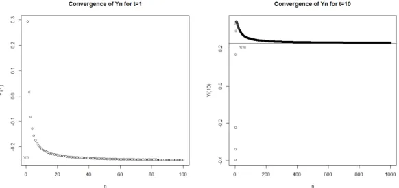
Figure 2: Variations ofYn(t)for two values oft,nvarying, in regard with the limit valueY(t)
In Figure 1, we see that the most n is high, the nearest the curve Yn is close to the
curveY. As for Figure 2, it shows how, fortsmall (equal to 1) and thenthigher (equal to 10), convergence is reached. We can notice that the moretis high, the fastest convergence is reached.
References
423–451, Oxford, 2011.
[2] A. Boudou and S. Viguier-Pla. Relation between unit operators proximity and their associated spectral measures. Statist. Proba. Letters, 80:1724–1732, 2010.
[3] N. Dunford and J. Schwartz. Linear Operators. Interscience Publishers, New-York, 1963.