Ovidiu-Aurelian DETEȘAN
Abstract: The paper presents the path planning of RTTRR small-sized industrial robot in a process of microprocessor packing, as a final stage in a modern manufacturing line. The work cycle consists in ten work phases, each phase being divided in minimum three path segments. The planning method is the (4-3-4) polynomials method, whose aim is to determine the interpolation functions of the generalized kinematic parameters (coordinates, velocities and accelerations) with respect to time. Their union will represent the path of the industrial robot, corresponding to its work cycle.
Key words: robot path planning, (4-3-4) polynomials method, kinematic parameters, MATLAB.
1. INTRODUCTION
The path of a robot is determined by the initial and the final position and orientation of its gripper, which mark the first and last path segments (end segments). In order to avoid the collision with the external obstacles within the robot’s workspace, a finite set of intermediary points is added, defining the intermediary path segments. The path-planning of RTTRR small-sized industrial robot is analyzed in this paper. The robot was described from the CAD model perspective in [1]. Its workspace was modeled in [2]. The geometric and kinematic models are presented in [3], while the dynamic model de-termination is performed in [4] and [5]. The robot is intended to be implemented in a process of microprocessor packing. The work cycle and the operating cyclogram, along with the work phases division and description, are presented in [6]. The path planning of the robot may be achieved using interpolation polynomials, of a higher or lower degree, according to the restrictions required by the technological pro-cess the robot is implemented in. The methods of path planning described in [7], [8], [9], [10] make use of interpolation polynomials of the 3rd, 4th, 5th and 6th degree, for the time-variation of the generalized coordinates. These methods are referred as: (4-3-4), 5-(4-3-4)-5, (5-4-6), 3n with
restrictions, 3n without restrictions. The robot path of (4-3-4) type was implemented in [11] and applied to the robot Fanuc LR-Mate 100iB.
2. (4-3-4) POLYNOMIALS METHOD
In the case of (4-3-4) path planning method, the end segments are interpolated by 4th degree polynomials and the intermediary segments by 3rd degree polynomials (cubic spline functions). In order to apply this method, presented in detail in [7], [8] and [11], the work cycle of the robot must be split in phases, and each phase must be divided into at least 3 segments: two end segments and at least one intermediary segment.
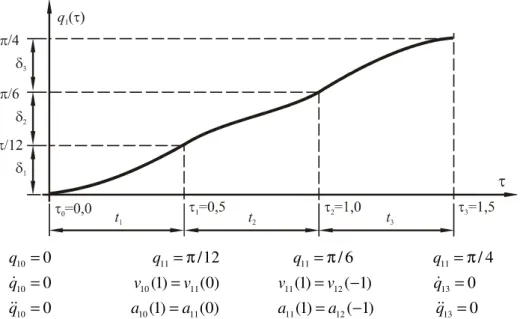
Fig.1 presents the dividing of the 1st phase of the robot’s work cycle on path segments, corresponding to the first joint (rotation). The first path segment is interpolated by time dependent polynomial of the 4th order. Because the generalized velocity is determined by deriving the generalized coordinate function with respect to time, the function needed to express it is a 3rd degree polynomial. The generalized acceleration will be expressed, consequently, by a 2nd degree polynomial. In the following equations, j=1,5 will denote the joint
0 ) 1 ( ) 1 ( ) 0 ( ) 1 ( 0 0 ) 1 ( ) 1 ( ) 0 ( ) 1 ( 0 4 / 6 / 12 / 0 13 12 11 11 10 10 13 12 11 11 10 10 11 11 11 10 = − = = = = − = = = π = π = π = = q a a a a q q v v v v q q q q q & & & & & &
Fig. 1. The 1st phase of the 1st joint work cycle of the RTTRR small-sized industrial robot The interpolation functions for the
generalized coordinate, velocity and acceleration specific to the first path segment, in the general case, are the following:
. ) 2 6 12 ( 1 ) ( ) ( ) 2 3 4 ( 1 ) ( ) ( ) ( ) ( 12 13 2 14 2 1 2 1 1 1 11 12 2 13 3 14 1 1 1 1 10 11 2 12 3 13 4 14 1 1 j j j j j j j j j j j j j j j j j j a t a t a t t t q t a a t a t a t a t t t q t v a t a t a t a t a t q t h + + = = + + + = = + + + + = = & &
& (1)
where
i i
t t= τ−τ−1
(2)
is the normalized time and it spans the interval [0,1]. The following notations are also used:
) (t
hji , the normalized interpolation polynomial
of the generalized coordinate, for joint j, segment i;
) (t
vji , the normalized interpolation polynomial
for the generalized velocity, corresponding to the joint j, segment i;
) (t
aji , the normalized interpolation polynomial
for the generalized acceleration, corresponding to the joint j and segment i;
jik
a , the polynomial coefficients corresponding to the joint j, segment i, and the kth order term
from the normalized polynomial function of the generalized coordinate (k =0,4 for end
segments, k =0,3 for intermediary segments).
The last path segment is interpolated by 4th degree polynomials also, but for a convenient determination of the polynomial coefficients, the following substitution is performed:
] 0 , 1 [ ;
1 ∈ −
− =t t
t . (3)
The generalized parameters polynomials become the following:
. ) 2 6 12 ( 1 ) ( ) ( ) 2 3 4 ( 1 ) ( ) ( ) ( ) ( 2 3 2 4 2 2 1 2 2 3 3 4 0 1 2 2 3 3 4 4 jn jn jn n n jn jn jn jn jn jn n n jn jn jn jn jn jn jn jn jn a t a t a t t t q t a a t a t a t a t t t q t v a t a t a t a t a t q t h + + = = + + + = = + + + + = = & & & (4)
Being expressed in the variable t=t +1, they
can be described as:
)]. 2 6 12 ( ) 6 24 ( 12 [ 1 ) ( ) ( )] 2 3 4 ( ) 2 6 12 ( ) 3 12 ( 4 [( 1 ) ( ) ( ) ( ) 2 3 4 ( ) 3 6 ( ) 4 ( ) ( ) ( 2 3 4 3 4 2 4 2 2 1 2 3 4 2 3 4 2 3 4 3 4 0 1 2 3 4 1 2 3 4 2 2 3 4 3 3 4 4 4 jn jn jn jn jn jn n n jn jn jn jn jn jn jn jn jn jn jn jn n n jn jn jn jn jn jn jn jn jn jn jn jn jn jn jn jn jn jn jn a a a t a a t a t t t q t a a a a a t a a a t a a t a t t t q t v a a a a a t a a a a t a a a t a a t a t q t h + − + + − + = = + − + − + + − + + − + = = + − + − + + − + − + + + − + + − + = = & &
one determines all the polynomial coefficients from the equations (1), (4) and (6). These coefficients are determined using the method exposed in [7], [8] and [11], by imposing, for each path segment, some restrictive conditions at both ends of each segment (initial and final restrictions), as well as continuity restrictions, in each intermediary point.
By combining all the restrictive conditions and using some coefficients which yield directly from the restrictive conditions, a system of 4+3(n-2) linear homogeneous equations can be set up. By solving this system, all the polynomial coefficients are determined. Replacing them into the equations (1), (4) and (6), the polynomials describing the generalized coordinates, velocities and accelerations are defined.
3. THE PATH PLANNING OF THE ROBOT
The above presented method will be applied in the case of the RTTRR small-sized industrial robot, implemented in a microprocessor packing process [6].
The joint j = 1 will be analyzed and the first phase will be split into n = 3 path segments, according to fig.1. The following initial conditions are imposed:
• at the moment τ0 =0:
0 ;
0 ;
0 10 10
10 = q = q =
q & && . (7)
• at the moment τ1=0,5s:
. 12 / ; 5 . 0 ; 12 / 10 11 11 0 1 1 11 π = − = δ = τ − τ = π = q q s t q (8)
• at the moment τ2 =1s:
. 12 / ; 5 . 0 ; 6 / 11 12 12 1 2 2 12 π = − = δ = τ − τ = π = q q s t q (9)
The vector of the remaining unknowns is:
T a a a a a a a
X1=[ 113 114 121 122 123 133 134] (12)
and the vector of the free terms is:
− + δ + − δ − − − − − δ = 3 13 2 3 13 13 13 13 3 13 12 10 10 1 10 1 10 2 1 10 11 1 2 1 2 1 t q t q q q t q q q t q t q t q B & & & & & & & & & & & & & & & &
. (13)
The matrix of the unknowns’ coefficients is given numerically by:
= 1 1 0 0 0 0 0 48 24 24 8 0 0 0 8 6 6 4 2 0 0 0 0 1 1 1 0 0 0 0 0 8 0 48 24 0 0 0 0 2 8 6 0 0 0 0 0 1 1 1
A . (14)
The unknowns’ vector is determined using the matrix equation:
1 1 1 A1 B
X = − ⋅
, (15)
Fig. 2. Interpolation functions graphs, for the joint 1, phase 1, segment 1, in normalized time
The following unknown polynomial coefficients are determined:
. 3927 . 0
6545 . 0 ;
2618 . 0 ;
3927 . 0
3927 . 0 ;
3927 . 0 ;
6545 . 0
134
133 123
122
121 114
113
=
= =
− =
= −
= =
a
a a
a
a a
a
(17)
By replacing the coefficients determined in (11) and (17) into the equations (1), (4) and (6), the interpolation polynomials for the given task, corresponding to the first phase of the first joint of the robot are obtained.
The first segment (τ0 →τ1) is characterized
by the functions:
). 9270 . 3 7124 . 4 ( 5 . 0
1 ) (
) 9635 . 1 5708 . 1 ( 5 . 0
1 ) (
6545 . 0 3927 . 0 ) (
2 2
11
2 3
11
3 4
11
t t
t a
t t
t v
t t
t h
⋅ + ⋅ − =
⋅ + ⋅ − =
⋅ + ⋅ − =
(18)
The following functions describe the second path segment (τ1→τ2):
Fig. 3. Interpolation functions graphs, for the joint 1, phase 1, segment 2, in normalized time
. 9270 . 3 5 . 0
1 ) (
9635 . 1 5 . 0
1 ) (
6545 . 0 ) (
2 12
2 12
3 12
t t
a
t t
v
t t
h
⋅ ⋅
=
⋅ ⋅
=
⋅ =
(19)
The third segment (τ2 →τ3) is described by
the interpolation polynomials below:
). 9270 . 3 7124 . 4 ( 5 . 0
1 ) (
) 9635 . 1 5708 . 1 ( 5 . 0
1 ) (
7854 . 0 6545 . 0 3927 . 0 ) (
2 2
13
2 3
13
3 4
13
t t
t a
t t
t v
t t
t h
⋅ +
⋅ =
⋅ +
⋅ =
+ ⋅ +
⋅ =
(20)
Fig. 4. Interpolation functions graphs, for the joint 1, phase 1, segment 3, in normalized time 4. CONCLUSIONS
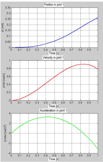
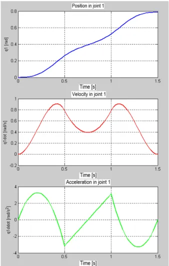
For a serial robot, the path can be defined as the union of the polynomial functions describing the time variation of the generalized coordinates, velocities and accelerations for each joint, during the work cycle. Because of the limited extents of this paper, this work presents only the functions operating the first joint of the robot, in the first phase of the technological process. After determining all the functions for all the joints in all the work phases of the process, one can say that the path planning is complete. In this case, having three kinematic parameters, five joints, ten phases each with minimum three segments, this leads to a number of minimum 450 functions in normalized time and 150 functions in real time. In this study, all the functions corresponding to the first two phases of the technological process, for all the robot joints are determined, using a script written in MATLAB, based on the function inter434() described in [8].
Fig. 5. First phase of the work cycle for the joint 1, in real time
5. REFERENCES
[1] Deteşan, O.A., CAD Model of the RTTRR Modular Small-Sized Serial Robot, Acta Technica Napocensis, Series: Applied Mathematics, Mechanics and Engineering, vol. 60, no. 1, pp. 69-74, Cluj-Napoca, 2017, ISSN 1221-5872.
[2] Deteşan, O.A., Workspace Determination for the RTTRR Modular Small-Sized Serial Robot, Acta Technica Napocensis, Series: Applied Mathematics, Mechanics and Engineering, vol. 60, no. 1, pp. 75-78, Cluj-Napoca, 2017, ISSN 1221-5872.
[3] Deteşan, O.A., The Geometric and Kinematic Model of RTTRR Small-Sized Modular Robot, Acta Technica Napocensis, Series: Applied Mathematics, Mechanics and Engineering, vol. 58, no. 4, pp. 513 - 518, Cluj-Napoca, 2015, ISSN 1221-5872.
Iterations Outwards and Inwards the Robot’s Mechanical Structure, Acta Technica Napocensis, Series: Applied Mathematics, Mechanics and Engineering, vol. 59, no. 1, pp. 25 - 32, Cluj-Napoca, 2016, ISSN 1221-5872
[5] Deteşan, O.A., The Dynamic Model of RTTRR Serial Robot – The Determination of the Generalized Driving Forces, Acta Technica Napocensis, Series: Applied Mathematics, Mechanics and Engineering, vol. 59, no. 1, pp. 33 - 38, Cluj-Napoca, 2016, ISSN 1221-5872.
[6] Deteşan, O.A., The Implementation of RTTRR Small-Sized Robot in a Processor Packing Process, Academic Journal of Manufacturing Engineering 15(1), pp. 91-96, Cluj-Napoca, 2017, ISSN 1583-7904.
[7] Negrean, I., Duca, A., Negrean, C., Kacso, K., Mecanică avansată în robotică (En: Advanced Mechanics in Robotics), Cluj-Napoca, UT Press, 2008, ISBN 978-973-662-420-9.
[8] Deteşan, O.A., Cercetări privind modelarea, simularea şi construcţia miniroboţilor (En:
Research Regarding Modeling, Simulation and Building of Minirobots), Ph.D. Thesis, Technical University of Cluj-Napoca, 2007. [9] Kacso, K., Negrean, I., Schonstein, C., The
Modeling of Working Process of the Serial Structure Fanuc, Acta Technica Napocensis, Series: Applied Mathematics and Mechanics, vol. 55, no. 3, pp. 725-732, Cluj-Napoca, 2012, ISSN 1221-5872.
[10] Negrean, I., Mura-Cozma, S.M., Negrean, D.C., Kacso, K., Formulations on Polynomial Functions in Robotics, Academic Journal of Manufacturing Engineering 7(3), pp. 66-71, Cluj-Napoca, 2009, ISSN 1583-7904.
[11] Deteşan, O.A., The Path Planning of Industrial Robots Using Polynomial Interpolation, with Applications to Fanuc LR-Mate 100iB, Acta Technica Napocensis, Series: Applied Mathematics and Mechanics, nr. 56, vol. IV, pp. 665-670, Cluj-Napoca, 2013, ISSN 1221-5872.
[12] FANUC Robot Series, R-J3iB Mate Controller, LR Handling Tool, Operator's Manual, B81524EN/02, 2006.
Planificarea traiectoriei minirobotului industrial RTTRR implementat într-un proces de ambalare a microprocesoarelor
Rezumat: Lucrarea prezintă planificarea traiectoriei minirobotului industrial RTTRR implementat într-un proces de ambalare a microprocesoarelor, ca etapă finală într-o linie modernă de fabricație. Ciclul de lucru constă în zece faze, divizate fiecare în minim trei segmente de traiectorie. Ca metodă de planificare a traiectoriei se folosește metoda polinoamelor de interpolare de tipul (4-3-4), a cărei scop este determinarea funcțiilor de interpolare a parametrilor cinematici generalizați (coordonate, viteze și accelerații) în raport cu timpul. Reuniunea acestora va reprezenta traiectoria robotului industrial, corespunzătoare ciclului de lucru al acestuia.