Negra sill
Ashley D Foguel1 and Jonathan Lees1
1Department of Geological Sciences,
University of North Carolina at Chapel Hill,
Abstract.
Understanding where shallow low velocity zones function is important in
assessing their relationship to eruption history. In Sierra Negra, a basaltic
shield volcano in the Galapagos Islands[Delaney, 2006] that has experienced
extraordinary uplift, the results of a combination of InSAR and CGPS data
suggest the existence of a sill at roughly 2 km depth. I believe this sill is, in
part, responsible for the areas uplift [Chadwick, 2006] by allowing release of
strain through faulting. To find both the thickness and velocity of the sill,
as well as, shed light on its relationship to uplift, I created a model of the
sill with varying thickness and velocity. I found the best fit of the model to
1. Introduction
Sierra Negra is located on Isabela Island, the largest island in the Galapagos Islands.
The summit of Sierra Negra is entirely occupied by a shallow elliptical caldera [Reynolds,
1995] (Fig. 1).
The summit has experienced nearly 5 m of total uplift since 1992, which is the largest
precursory inflation ever recorded at a basaltic caldera. This large uplift was
accom-modated by at least three trapdoor faulting events, taking place in January 1998, April
2005, and October 2005. The events occured about 3 km south of the center of a shallow
low velocity zone, which was first discovered through InSAR data [Jonsson, 2005]. I
be-lieve this shallow low velocity zone accommodated the trapdoor faulting, which rebe-lieved
accumulated strain and, thus, postponed eruptions [Jonsson, 2005].
Along with first locating the existence of the shallow low velocity zone, the InSAR data
also suggested that the low velocity zone was a sill at roughly 2-2.2 km depth. While
tomographic imagining was able to soundly map the caldera and large magma chamber
at depth, it was unable to map the shallow low velocity zone.
Mapping the thickness and velocity of the low velocity zone is key to gaining insight
into the effect the sill has on both eruption history and uplift processes, as well as, to a
better understanding of the activity and hazards associated with Sierra Negra and other
shallow low velocity zones.
2. Background on the Model: Why a sill?
InSAR data was used to determine the vertical and horizontal components of
was consistent with a sill-like shape for the low velocity zone underneath the caldera, as
opposed to spherical or stock-like bodies [Yun, 2006], I felt confident using a sill model.
3. Methods
The first model was created without the introduction of real seismic data. I used E3D
to propogate 2D waves through a described subsurface, ranging from a solid block with no
magma chamber to a solid block with a shallow low velocity zone, in which the parameters
of run-time, source functions, velocity model, and grid structures were generated using R.
The first model had two separate components: one, a model with changing thickness,
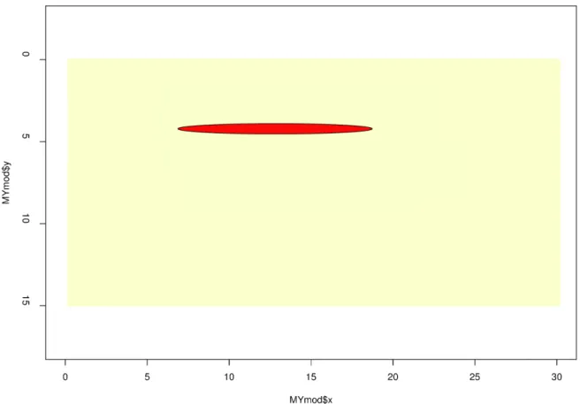
and the second, a model with varying velocity. For the thickness model, waves are
pro-pogated through a field with no low velocity zone to a field with a sill-shaped 4.5
km/sec-velocity zone the area of the entire plane (Fig. 2).
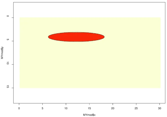
For the velocity model, waves are propogated through a plane with an oval 4 km thick,
which first had the same velocity as the plane and then has increasingly lower velocities
(Fig. 3). The initial values of 4.5 km/sec for the thickness model and 4 km thick for the
velocity model were chosen based on average thicknesses and velocities for other shallow
low velocity zones in hot spots.
The synthetic seismograms are then animated at each thickness and velocity interval,
ranging from no low velocity zone (Fig. 4) to a large low velocity zone (Fig. 5).
To be able to compare the synthetic seismograms with real seismic data I created a
second model. The second model incorporated the synthetic seismograms created in E3D
with the real data from the stations and earthquake locations around Sierra Negra (Fig.
The model was created by finding a seismic event in the real seismograms then
propagat-ing a simple version of that same event through E3D and projectpropagat-ing the real seismograms
on the cross-sectional cut used in the model (Fig. 7). To improve the match, I only
projected seismograms that were close to the synthetic source, usually able to use only
2-4 of the stations available, and filtered the chosen data.
3.1. Analysis of the waves in the models
Figure 4 is the ideal propogation of waves assuming no shallow low velocity zone. In
the figure, we clearly see the first arrivials (the primary waves), followed by the second
arrivials (the secondary waves), and then finally followed by the surface waves, whose
arrivals fall at a steeper slope.
In comparison, figure 5 has a large low velocity zone. While the primary wave and
secondary wave arrivals are still apparent, though morphed, the other arrivals show a
criss-crossing pattern.
This criss-cross pattern is due to the waves created by the source propogating through
the model with some ray paths penetrating and other ray paths missing the shallow low
velocity zone. The ray paths that miss the low velocity zone reach the surface faster than
the ones that penetrate the low velocity zone, making some ray paths that are further
from the source arrive before ray paths closer to the source. Furthermore, a ray path
entering a low velocity zone acts as a ray path entering any other discontinuity, meaning
that the wave creates both a reflected and a refracted wave upon hitting the low velocity
zone. Also, the refracted wave creates another reflected and refracted wave when it hits
the upper boundary of the low velocity zone, which creates another refracted and reflected
This disruption of arrival times in relation to the distance from the source is what
creates the observed criss-cross pattern seen in both the model and the real seismograms
(Fig. 6A).
3.2. Finding the best model
To find the conditions under which the synthetic seismograms most closely match the
real seismograms, I calculated the RMS residual of the real seismogram to the closest
synthetic seismogram for each station on each cross-sectional cut, using the following
equation:
rms=q(real−predicted)2 (1)
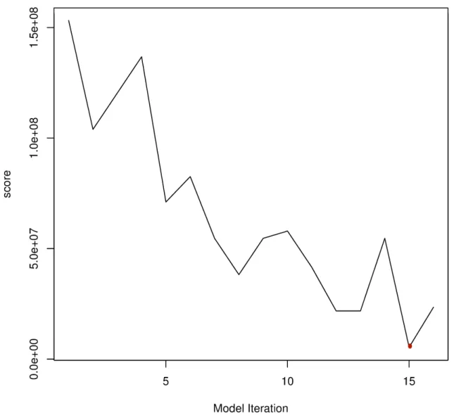
For the calculation, I used three parameters: time, thickness, and velocity. To find the
minimum difference, I added up the score for each point on the compared wiggles and
found the compared wiggle set with the sum closest to zero for all 35 iterations of my
model. I found the best model to be at the 15th model iteration (Fig. 8), which placed
the sill at 6km thick with a velocity of 4.29km/sec.
4. The future of the project
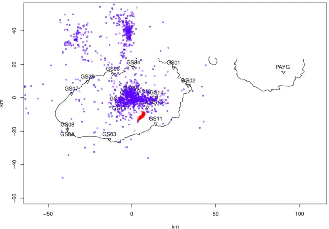
However, the real data is very complex, so it is hard to know if the match up is due
to signal or noise. To test the cause of the match, I have started locating clusters in the
real data (Fig. 9). I plan to stalk the clusters then re-project them and find new the new
RMS residuals for the real stalked seismic data with the synthetic data.
As a further measure to improve our confidence in the match, I plan to add more
of stations within proximity of the caldera. In any case, a small number of stations put
into question any observed correlation.
5. Conclusion
Before comparing the synthetic seismograms with recorded seismograms, the effects of
varying velocity and thickness of the sill in model were tested. The tests were run with
thicknesses ranging from about 2 to 6 kilometers and velocities ranging from about 6 to
4km/sec at the suspected depth of 2 kilometers.
As expected, the resulting animations showed that at greater sill thicknesses and higher
sill velocities the larger the deformation of the waves.
The second model, which incorporated the real seismic data with synthetic data, showed
some matching. Looking at the RMS residuals, I determined the best match to place the
sill at 6km thick with a velocity of 4.29km/sec; however, it was hard to tell if the matching
was due to noise in the signal, the real signal, or the small sample size. To test if either
noise or the complexity of the real signal in comparison to the simplistic and idealized
real signal were the cause of the mismatch, I found clusters in the real seismic data. Next
I plan to stalk the data and see how the real seismograms and the synthetic seismograms
match.
Acknowledgments. The authors thank Keehoon Kim and Daniel C. Bowman for their
insightful conversations that resulted in script efficiency improvements. I would also like
to thank the Lees Mitchel Laboratory of the University of North Carolina at Chapel Hill
References
Chadwick, William, Dennis Geist, Sigurjon Jonsson, Michael Poland, Daniel J. Johnson,
and Charles M. Meertens. ”A volcano bursting at the seams: Inflation, faulting, and
eruption at Sierra Negra volcano, Galapagos.” Geological Society of America. 34.12
(2006): 10258.
Delaney, John, Wayne Colony, Terrence Gerlach, and Bert Nordlie. ”Geology of
Vol-can Chico Area on Sierra Negra VolVol-cano, Galapagos Islands.” Geoscience World. 84.7
(2006): 2455-70.
Jonsson, Sigurjon, Howard Zebker, and Falk Amelung. ”On trapdoor faulting at Sierra
Negra volcano, Gala pagos.” Elsevier. 144. (2005): 59-71.
Jonsson, Sigurjon. ”Stress interaction between magma accumulation and trapdoor faulting
on Sierra Negra volcano, Galapagos.” Elsevier.471. (2009): 36-44.
Reynolds, Robert, Dennis Geist, and Mark Kurz. ”Physical volcanology and structural
development of Sierra Negra volcano, Isabela Island, Gal apagos archipelago.”Geological
Society of America. (1995): 1398-410.
Yun, S., P. Segall, and H. Zebker. ”Constraints on magma chamber geometry at Sierra
Ne-gra Volcano, Gala pagos Islands, based on InSAR observations.”Journal of Volcanology
Figure 2. The model of the subsurface of the caldera with a flattened oval in a plane
with depth in kilometers on the y-axis and distance from the source on the x-axis. The
Figure 3. The model of the subsurface of the caldera with a thick oval in a plane with
depth in kilometers on the y-axis and distance from the source on the x-axis. The waves
Figure 4. Synthetic seismograms with no low velocity zone with time in seconds on
the y-axis, stations on the upper x-axis, and distance in kilometers on the lower x-axis.
Figure 5. Synthetic seismograms with a sizeable low velocity zone with time in seconds
on the y-axis, stations on the upper x-axis, and distance in kilometers on the lower x-axis.
Figure 7. (A) Real seismic data projected onto a cross-sectional cut through Sierra
Negra with time in seconds on the y-axis, stations on the upper x-axis, and distance
in kilometers on the lower x-axis. These seismograms reflect the ray paths of both the
synthetic seismograms and the real seismograms once they reach the surface. (B) Real
Figure 8. The RMS residuals for only the first 16 model iterations with the minimum