The Impact of Motherhood, Childcare, and Location on Women’s Wage
Growth
By: Audra Killian
March 2017
Economics Department
The University of North Carolina at Chapel Hill
Approved:
Abstract
This paper examines how motherhood, the use of childcare, and an individual’s geographic location affects their wages for a fifteen year period using cross-sectional data. Incorporating Gary Becker’s theory on the Gender Division of Labor (1985) and the feminist theory of the ‘second shift’, the paper aims to better understand how wages are affected, and what factors contribute to that change. This paper also evaluates how an individual’s location, which highly corresponds to their ideological values, affects their wages. By utilizing the NLSY79, this
Acknowledgments
I. Introduction
The gender wage gap is a real economic problem. Despite the fact that over the last several decades women have been entering the workforce in record high numbers and have made huge strides in educational attainment, women’s wages have stagnated (Council of Economic Advisors, 2014; BLS, 2016). Compared to men, women are paid less, more likely to hold low-income jobs, and more likely to live in poverty. This not only hurts American women, but also American families. There is no sector of the economy, education level, or profession that does not have this gender wage disparity. A variety of reasons could explain this inequity, however current research has indicated that one of the largest reasons for wage inequality is motherhood (Fuchs, 1988).
This paper will focus on the effect of the number of children and the use of childcare on a woman’s wages over a fifteen-year period of time. Even though it has become acceptable for women to step outside the rigid stereotype of the complacent housewife, they are still expected to be the primary caregiver for their children. Despite the popular rhetoric that encourages men to have a larger role in the household, women are still more likely to do the majority of cleaning, cooking, and child rearing than men. This has been termed by mainstream feminists as ‘the second shift,’ which may cause women to be less motivated and active in the workplace, thus reducing their ability to work at the same level as their male peers (Budig and England, 2001). This combined with subconscious prejudices against mothers, markets and employers have enacted ‘motherhood penalties’ that take the form of missed promotions or employment
wage. So when women re-enter the workforce, they are unable to achieve the same level of success as their male or childless peers.
In comparison, working fathers are often paid more, even with similar credentials and experience. Though this inequality may seem to only affect women, it drags the entire American economy down: current research has found that if women were to achieve equal gender parity by 2025, the US government could add 4.3 trillion dollars to the economy (Ellingrud et al., 2016). So it is beyond imperative that we figure out what is truly causing these low wages, and determine if there are any possible ways to alleviate it.
While there is an extensive amount of literature on the relationship between women’s wages and children, this paper will also differentiate from past literature by including a control for whether or not an individual has reliable childcare for their first child. Accessible childcare is common in a large portion of developed countries, including France and Sweden, and operate in a variety of ways, including vouchers, state provided care, or legislation requiring private companies to provide some sort of care themselves. Though countries with better childcare policies than the US still have a gender wage gap, wages have grown over the past three decades, while workers’ wages in the US have continued to stagnate (European Union, 2016). The model will also differentiate between the types of childcare, and the effect they have on women’s wages, specifically, the effect of paid childcare on women’s wages.
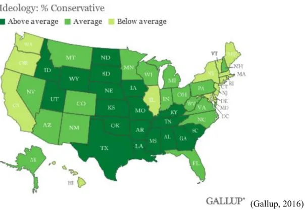
government, and thus less government assistance; or an indication of economic instability, where a particular region may have lower wages and less economic growth. Regional discrepancies in wages could indicate widespread gender inequity in the workplace, which would call for policy reform. However, it is important to note that not all individuals have the same beliefs as their peers, so using regional location does not necessarily dictate their personal beliefs.
Figure 1: Percentage of Conservative Ideology by State
an even smaller population. The West is characterized by liberal political ideology, a diverse population, and a diverse job market (Desilver, 2014).
This paper will also analyze the urban or rural location of the individuals in this study, and the effect it has on their wages. Since more urban areas tend to have more public services as well as better public transportation, individuals have better access to a wider array of careers and jobs. In more rural areas, there tends to be a more homogeneous labor market. Past research has indicated that individuals who hold more conservative beliefs would prefer to live in small towns in rural areas, while those with more liberal beliefs prefer to live in more urban areas, which are comprised of more diverse families and individuals (Desilver, 2014). These ideological beliefs affect how an individual raises her family, how many children she prefers, and whether she participates in the labor force. So, whether a woman lives in an urban area affects her familial decisions, thus affecting her wage.
This paper will also differentiate from past analysis of mothers’ wages by using family beliefs as the exclusion variable in two Heckman models. Past research has used the cost of transportation to work or distance traveled as the differing variable in the first stage for selecting whether or not an individual enters the labor force. Instead, both models use variables that indicate an individual’s personal beliefs about the role of women or the importance of traditional values as exclusion variables, assuming that these conservative or liberal beliefs would affect whether an individual enters the labor force or chooses to become a mother, but does not affect their wages.
research, with similar magnitude and direction of past papers, and the second finding indicates that mothers who have reliable, childcare (paid or school) have higher wages. This study also found that mothers in urban cities have higher wages, which matches assumptions since urban areas tend to have better transport and a wider array of job opportunities. Similarly, individuals who live in the Northeast, which is characterized by urban areas, earn more over time as well.
In the following section, I will discuss past literature in economics on the growth of mother’s wages and a few past papers on the feminist theory behind the wage gap. In section III, I will describe the cross-sectional data set used in my empirical model, as well as evaluate the summary statistics for the relevant variables. Section IV presents and explains the theoretical model of an individual’s decision process of having a child. Then I apply the theory from the model to four separate regressions for the empirical model in Section V. Results are presented in Section VI and a policy recommendation is given in Section VII based off of the results and past research. Concluding remarks will be given in Section VIII, and figures and tables are given in the appendix.
II. Literature Review
Over the past three decades there has been an extensive amount of research on the relationship between motherhood and wages, both empirical and theoretical. The wage
found that implementing wage equality legislation does little to better the gap, and instead the government needs to create policies that provide maternity leave and accessible childcare, and encourage flexible working hours. Budig and England used the NLSY82 data to estimate a fixed effects model; they found that there is a 7 percent wage penalty per child, and that the penalty is larger for married women than for unmarried women. While they controlled for children and part-time work, they theorized that the penalty most likely results from the effects of motherhood on productivity or from discrimination from employers.
Correll et al. (2007) found that in hiring situations, obvious factors indicating motherhood, such as PTA meetings, are correlated with lower salaries and fewer employment offers for women, which they term as “motherhood penalties.” Biological fertility events, sex ratios and twins, were used by Angrist and Evans (1998) as instrumental variables for the number of children in the wage equation; they found that after 13 years of age, the additional child no longer affects a woman’s income, and never affected a man’s in the first place. Their IV estimates are significant but smaller than the estimates from OLS; the IV estimates were also small for educated women and were shown to have no impact from family size on the husband’s supply of labor.
heterogeneity leads to biased estimates of marriage and motherhood on wages. Their use of instrumental variables suggests that normal OLS cross-sectional and first estimates understate the direct effect of children on wages.
Motherhood delays have also been a popular topic of research in the past few decades. Chandler et al. (1994) used OLS to find that with each year of motherhood delay, individuals gain 1% of wage increase, however their IV estimates are sensitive to specification and are deemphasized in their results, indicating the weakness of their chosen IVs, ‘beliefs.’ Amuedo-Dorantes and Kimmel (2003) found that delaying motherhood after 30 eliminates the family gap altogether, contrasting with previous research by Blackburn et al. (1993), which found
motherhood had no effect on earnings, despite using similar IVs. Amuedo-Dorantes and Kimmel utilize the NLSY79, where they focused on college-educated women and produced base-line results. They found that college-educated mothers do not experience the mother wage gap at all, and in fact, they experience a wage boost compared to college-educated childless women. They also found that a fertility delay enhances this wage boost, which the authors theorize stems from women searching longer for friendly work environments. In comparison, Blackburn et al. (1993)’s empirical model found that fertility delay and wages are positively correlated, where individuals delayed motherhood in order to attain the assumed proxies for human capital
(education, job experience), while when they tested for motherhood in general, they found that it affected wages very little.
she is given at her job. Becker theorizes that this could be due to exhaustion, a decreased dedication to their profession, or a revision of priorities, where a woman may become uninterested in receiving a promotion or raise. This agrees with the feminist theory of the “second shift,” which theorizes that instead of liberating women by a higher percentage of women entering the workforce, they are further inhibited by the increased amount of work (Correll et al., 2007). The amount of housework male partners contribute has not majorly increased over the past four decades, so women are still expected to the do the majority of the cooking, cleaning, and child rearing.
Though there is extensive research on the relationship between women’s wages and children, many papers only rely on one model, such as Fixed Effects or Two Staged Least Squares,
however they rarely comment on the selection bias present in the OLS. Most papers also only look at how a single child affects women’s wages, however intuitively, each child compounds the work a mother has in her home as well as her stress at work. Also, most papers only analyze the typical human capital characteristics associated with wages, so any other factor affecting how much they earn and whether they enter the labor market is ignored.
III. Data and Summary Statistics
For this paper, my econometric model will use the National Longitudinal Survey of Youth (1979), focusing on the observations from 1985-2000. This survey consists of panel data from 1979 to 2012; in 1979 at the time of their first interview, cohorts were 14-22 years old, and were 47-56 at the time of their last interview. 12,686 cohorts were interviewed in 1979, with both 50% female and 50% male. The data set’s cohorts are racially diverse, with 59.1% white, 25.01% black, and 15.88% Hispanic/Latino. The whole sample selection was randomly chosen through a multi-stage stratified area probability sample of dwelling units and group dwelling quarters in 1978, then individuals between the ages of 14-22 in 1979 were chosen. Respondents reside in all 50 states and the District of Columbia. The rate of retention for the survey from 1979 to 2000 is 90%, indicating very little attrition bias for the years selected for this model. The survey has thousands of questions on an individual’s education, family background, employment, fertility, beliefs and expectations, health, income, marriage, and children.
used in the models are given in Table 1 and variable definitions are given in Table 2.The summary statistics are for observations recorded for the years between 1985 and 2000.
Observations following the year 2000 are dropped because: 1) individuals rarely had a child in the final years of the survey and 2) since we are evaluating the effect of childcare on women’s wages, looking at how children over the age of 7 would not produce significant results. The average age of cohorts in this study is 30.5 for women, and over half of the individuals in the study live in urban areas. Slightly less than half of all those in the survey are women, and
compared to the total number of children individuals’ have, cohorts have slightly less children in their household. The average family income across panels is around 39,500 dollars and the average spousal wage is 27,500 dollars.
The statements on familial attitude indicate that the overall survey sample has fairly progressive views on family and the role of women in the house. For example, concerning whether it is better for women to work outside the home, more than half of the cohorts agreed, and concerning whether women belong in the home, over half disagreed with the statement. However, a question stating that it is better to maintain traditional roles for men and women in home, concerning homemaking and earning statuses, the average response was almost half agree and half disagree, which goes against the other average response given to the other attitude questions.
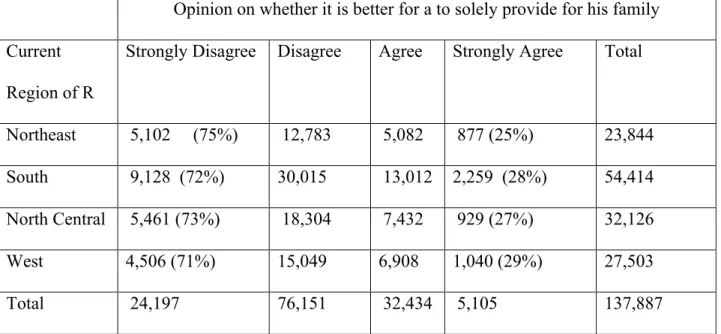
An interesting analysis of the data is found in Table 3, where the attitude variable on Traditional Roles is cross summarization with the regional location of individuals (both male and female). This question was asked three times over the fifteen-year period of our model.
universities, and liberal political ideology. However, when compared to the other regions, the Northeast did not hugely differ from the responses given; 75% of all cohorts in the Northeast disagreed with the statement, while the other three regions deviated by at most 4%, with 71% of individuals in the Western region disagreeing with the statement. Surprisingly, the Southern Region did not widely differentiate from the Northeast, despite of the fact that the South is usually stereotyped as more traditional.
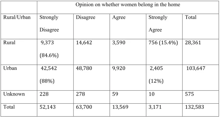
Another interesting analysis is the cross summarization of an attitude variable on the role of women with the urban/rural location of individuals (both male and female), located in Table 4. There is almost four times as many individuals in urban areas compared to rural areas, and 88% of individuals in urban areas disagreed with the statement compared to the 84% of individuals in rural areas. This agrees with the commonly progressive views common in urban areas, where due to the higher population, the city government may provide better public services. Individuals in rural areas are usually characterized as being more conservative, as well as more likely to work in agriculture and manufacturing. However, the small difference may be due to how the survey calculated an urban area, where they divided the urban population of a county by the total county population and multiplied it by 100. They then characterized a county as rural when the urban population is less than 49%. So this may have categorized more rural-like counties as urban, possibly skewing the data.
offers a large amount of information on a diverse set of cohorts. If the selection bias can be controlled for, NLSY is the best available data source for the goals of this paper.
IV. Theoretical Model
The theoretical model for this paper is illustrating the decision-making process of an individual, concerning whether or not to have a child. It can be assumed that individuals who have children receive utility from having a child (K), attaining consistent, reliable childcare (Q), and a vector of other consumable goods (X). Reliable childcare can be defined as paid services, such as a preschool, nursery, or babysitter, as well as another regular arrangement, such as a playgroup or in a relative’s care. In this equation, Q is total quality childcare, and at the current moment, the fixed price of quality childcare is 0, so PQ=0.
It can be assumed that when an individual has a child, she acts as an altruistic economic actor, whose utility is maximized when her child’s utility is maximized, which is done through a combination of income from her employment and time spent with her child. All demands and preferences are identical across all individuals. In this model, having a child provides an
individual with a large amount of utility, which is why they may choose to reproduce despite the high costs. The comparison of utilities of two otherwise identical individuals, one who chooses to reproduce (K1) and one who chooses to not reproduce (K0), given the costs children, care, and
other goods, can be illustrated by:
U1(𝐾!,𝑄!,𝑋!| PK, PQ(1), PX)>U0(𝐾!,𝑄!,𝑋!| PK, PQ(0), PX) (1)
Whether or not an individual chooses to have a child and how many to have ultimately depends on an individual’s objective to maximize lifetime utility:
𝑢(𝐾!,𝑄!,𝑋!) !
!!!
where 𝑇 is the end of life.
The utility function of a woman facing the decision of having a child can be illustrated by:
𝑉∗ 𝑝!,𝑚! =U 𝐾!,𝑄!𝑋! (3)
Where Q is total quality, or individual quality of children multiplied by the number of children, and the equation is a function of various prices (p) and income (m). In each different time period, t, an individual may receive a different amount of utility from having a child or from the amount of care they use. The individual makes decisions considering a budget constraint, illustrated by:
𝑃!!𝐾+𝑃
!!𝑄+𝑃!!𝑋=𝑚!𝐸!+𝑁! (5)
Which consists of the price of children (𝑃!!), which includes food, clothing, and other
necessities, the price of childcare (𝑃!!), most likely monetary even though these services could be
exchanged for items or services, and the price of X (𝑃!!). The individual’s income employment
status is represented by 𝐸!, income is represented by 𝑚!, and non-earned income is represented by 𝑁!. The utility function maximizes K, X, and Q, subject to the budget constraint.
The corresponding expenditure model consists of:
eH(v, p)= 𝑃!!K+𝑃!!X+PQQ (6)
and
U(Kt, Qt, Xt)≥ v (7)
Where the individual minimizes the cost of K, X, and Q in order to achieve her given utility function. All Hicksian demands of this expenditure model are downward sloping and symmetric in their cross-price effects.
have a preference not to have a child, which cause them to have higher utility from not having a child:
U1(𝐾!,𝑄!,𝑋!| PK, PQ(1), PX)<U0(𝐾!,𝑄!,𝑋!| PK, PQ(0), PX) (8)
However, it is difficult to illustrate different preferences, whether they are due from societal pressure or just personal choice, which is why this model operates on the assumption that all individuals have homogenous preferences. Another limitation is that this model only operates under the assumption that this is an individual’s first child, or that if the individual already has a child, this would not affect their choice to have another child.
This model predicts that when women maximize their utility by having children they simultaneously increase the income needed to provide for their child, assuming that they are acting in the best interest of their child, as well as decrease their income by having to pay for childcare and by taking time off in order to care for their child. By obtaining childcare, their wages theoretically would go up, however their expenses would also increase. The empirical model will test how much children will affect women’s wages, as well as if childcare can increase their wages, which would allow the individual to pay for childcare in the future.
V. Empirical Model
𝑙𝑛𝑊𝑎𝑔𝑒!,!!!" =𝛽!+𝛽!𝑛𝑢𝑚𝑐ℎ𝑖𝑙𝑑ℎℎ!,!!!+𝛽!𝑆𝑐ℎ𝑦𝑟𝑠!,!!!"+𝛽!𝐸𝑥𝑝!,!!!"+𝛽!𝐸𝑥𝑝!,!!!"! +
𝛽!𝑅𝑎𝑐𝑒!,!+𝛽!𝐶ℎ𝑖𝑙𝑑𝑐𝑎𝑟𝑒𝑎𝑟𝑟𝑎𝑛𝑔𝑒!,!!!"+𝛽!𝑌𝑒𝑎𝑟! +𝛽!𝑀𝑎𝑟𝑟𝑖𝑒𝑑!,!!!"+𝛽!𝑅𝑒𝑔𝑖𝑜𝑛!,!!!"+
𝛽!"𝑈𝑟𝑏𝑎𝑛!,!!!"+𝜈!,! (9)
Where the subscript i represents the economic actor in this model, an adult woman, the subscript t is the time period of 1985, when all of the models begin to evaluate individuals, and the
subscript t+15 indicates the variables that represent relevant information recorded fifteen years after original time, t.
The independent variable, 𝑛𝑢𝑚𝑐ℎ𝑖𝑙𝑑ℎℎ!,!, is a continuous variable that indicates the
number of children an individual has. Evaluating the relationship between the number of children in an individual’s household and her wages is based off of Becker’s theory of the Gender
Division of Labor, where each additional child causes an increase in household work, thus increasing a woman’s overall work load, which may decrease the energy an individual could devote to their job. 𝑆𝑐ℎ𝑦𝑟𝑠!,!!!" is a continuous variable that represents an individual’s highest
level of education attained, where 12 indicates a completion of high school and 16 indicates a completion of a four year college; 𝑅𝑎𝑐𝑒! is a binary variable representing the an individual’s race, where 1 indicates Hispanic, 2 indicates black, and 3 indicates non-hispanic, non-black; and the two work experience variables, 𝐸𝑥𝑝!,!!!" and 𝐸𝑥𝑝!,!!!"! are continuous variables which
represent the length of time, measured in years, an individual has spent in the labor market. These two variables represent relevant past experience.
𝐶ℎ𝑖𝑙𝑑𝑐𝑎𝑟𝑒𝑎𝑟𝑟𝑎𝑛𝑔𝑒!,!!!" is a categorical variable that describes the type of childcare used
other than their own home, five if youngest child is cared for in their own home by a parent or a relative, six if the individual works at home, and seven if the mother takes her youngest child to work. Since this variable includes paid forms of childcare, daycare and preschool, the model may be endogenous due to the reverse causality that exists the in the relationship between childcare and wage. The ability to pay for childcare may only be accessible for those that already earn higher wages than average, so the coefficient on the childcare variable may be biased. Though the bias is known, it is difficult to account for it in the model, especially since there are no instruments in the NLSY79 that would affect the use of childcare and not an individual’s wages.
The model also includes a marriage variable, 𝑀𝑎𝑟𝑟𝑖𝑒𝑑!,!!!", which is a categorical
variable that indicates an individual’s marital status, where the variable equals zero if the individual has never married, one if the individual is currently married, two if the individual is currently separated, three if the individual is currently divorced, and four if the individual is widowed. The effect of marital status on women’s wages is fairly ambiguous and no past
research has definitely indicated its impact, whether women experience a boost or a penalty, and whether that result is statistically significant (Western & Hewitt, 2005).
There are two geographical variables, 𝑅𝑒𝑔𝑖𝑜𝑛!,!!!" and 𝑈𝑟𝑏𝑎𝑛!,!!!", which evaluate the
individual’s location and what effect that has on their wages; the former variable is categorical and indicates what region of the US the individual lives in, where one indicates that the
individual lives in the Northeast, two indicates that the individual lives in the North Central part of the US, three indicates that the individual lives in the south, and four indicates that the individual lives in the Western US. This variable could infer a variety of things about
become a mother or to enter the workforce. The second geographic variable is binary and indicates whether an individual lives in a rural or urban area. Whether or not an individual lives in an urban area could affect their wages as well as their access to childcare; since more urban areas often offer better public services and public transportation, which allows for women to access work easier and may require them to work for higher wages due to higher taxes. Also, compared to more rural areas, where there may be homogeneity in terms of possible jobs and careers, cities offer a diversity of possible fields, which allow for a wide range of salaries and wages. Finally, the mean of the error term, 𝜈!,!, has an expected value of zero given values for
the independent variables:
𝐸 𝜈!,! 𝑥! =0 (10)
An interesting element of the survey is that despite the dozens of questions on childcare, none are posed towards the male cohorts of the study. So while it would be interesting to
evaluate the relative effect of childcare on both men and women’s wages, this paper is only able to measure its relationships with women’s wage growth. This omission illustrates possible stereotypes and assumptions that were incorporated into the study. Those implemented the study may have assumed that men may not know about their child’s care arrangements or that the location and caregiver of children was only a woman’s job. Nevertheless, this omission excludes single fathers as well as individuals in gay relationships.
This model does not control for the sample selection bias that is present due to an
wage and the independent variable representing whether or not an individual has had a child. In this relationship, future wages could affect when and how many children a woman has, and a child could affect a woman’s wage growth over the years. Lastly, this model does not control for the effects of unobserved heterogeneity on the results; characteristics, such as preferences, productivity, or dedication, which often do not change over time, can affect wages, and these are not measured in the data set.
Heckman Selection Model for Labor Force Participation
In order to control for sample selection bias that stems from the choice an individual makes whether or not to enter the work force, this paper will use a Heckman selection model (Heckman, 1979). In the OLS, we are regressing the number of children they have on their wages, assuming that they every female individual is currently in the labor market. However, there are individuals every year who are not working or actively looking for work, so our results would be skewed because they were estimating the effect of children on individuals’ wages, which are zero. A Heckman model was used to account for this type of selection bias in Bar et al. (2015), Schafgans & Stelcnery (2006), and Prieto-Rodríguez & Rodríguez-Gutiérrez (2000).
The model considers that observations are ordered into two regimes, which are defined by whether an individual chooses to participate in the labor force. The first stage is the selector equation that defines the dichotomous variable, Labor Force Participation (LFP), indicating whether or not an individual participates in the labor force:
𝐿𝐹𝑃!,!!!"∗ =
𝛾!+𝛾!𝑌𝑒𝑎𝑟!+𝛾!𝐸𝑥𝑝!,!!!"! +𝛾
!𝐸𝑥𝑝!,!!!"+𝛾!𝑆𝑐ℎ𝑦𝑟𝑠!,!!!"+𝛾!𝑁𝑢𝑚𝑐ℎ𝑖𝑙𝑑ℎℎ!,!+
Where 𝐸𝑥𝑝!,!!!" and 𝐸𝑥𝑝!,!!!"! are both continuous variable representing an individual’s work
experience; 𝑁𝑢𝑚𝑐ℎ𝑖𝑙𝑑ℎℎ!,! is a continuous variable representing the number of children the
individual currently has in her household; 𝑆𝑐ℎ𝑦𝑟𝑠!,!!!" is a categorical variable indicating the
highest level of education completed by the individual; 𝑀𝑎𝑟𝑟𝑖𝑒𝑑!,!!!" is a categorical variable
indicating an individual’s marital status; 𝑅𝑎𝑐𝑒!,!!!" is a categorical variable indicating that the
race of the individual; and 𝑦𝑒𝑎𝑟! is a continuous variable indicating the current year of analysis. The exclusion variable, 𝑊𝑜𝑚𝑒𝑛𝑟𝑜𝑙𝑒!,!, represents a question posed to individuals in the survey,
on whether agree or disagree with the statement that “Women’s role is solely in the home.” The variable is binary and coded as one and two if they disagree with the statement and three and four if they agree with the statement. If an individual agrees with this attitude statement, this may affect their labor force participation, whether or not they stay at home as a housewife or enter the work force; however, whether they agree with this statement has little affect on her wage. The error term, 𝜇!, has a standard normal distribution.
𝐿𝐹𝑃!!!"∗ is a latent variable which indicates the utility from participating in the labor
force:
𝐿𝐹𝑃!,!!!"= 1 𝑖𝑓 𝐿𝐹𝑃!∗,!!!" >0 𝑎𝑛𝑑 𝐿𝐹𝑃! =0 𝑖𝑓 𝐿𝐹𝑃!,!!!"∗ ≤ 0 (12)
𝐿𝐹𝑃! is an indicator for labor force status and all of the independent variables in (11) are
determinants of this status. After estimating the parameter estimators using, the probit maximum likelihood method, the second stage of this model involves estimating an OLS regression of wages conditional on 𝐿𝐹𝑃! = 1 and a vector of observed explanatory variables (age, education,
chidcare, etc.), which will be denoted as x in the following equation for simplicity:
𝐸 𝑙𝑛𝑤𝑎𝑔𝑒!,!!!" 𝐿𝐹𝑃!,!!!"= 1,𝑥! = 𝛽!𝑥
! +𝐸 𝜀! 𝐿𝐹𝑃!,!!!" =1) =𝛽!𝑥! +𝐸 𝜀! 𝜇! > 𝛾!!𝑧!)
where 𝑤𝑎𝑔𝑒!,!!! is the dependent variable, measured as the amount of money an individual
earns annually from employment. 𝑥! represents the vector of independent variables of the second stage of this model, 𝑧! represents the determinants in (11), 𝛽! represents the parameter
estimates for the second stage independent variables, and 𝛾!! represents the parameter estimates for independent variables in (11). The degree that the normally distributed error term, 𝜀!, of the second stage regression equation is correlated with the error term, 𝜇!, of the probit equation is
represented by ρ. If we assume that the joint distribution of 𝜇! and 𝜀! is bivariate normal, the expected value of 𝜀!, conditional on 𝜇!, is:
𝐸 𝜀! 𝜇! >𝛾!!𝑧
! =𝜌𝜎!𝜎! !(!!
!!
!)
!(!!!!!) (14) where 𝜎! and 𝜎! are the error variances of the OLS and probit models respectively; 𝜎! is
unidentified, so it is set to 1. The bracket term, inverse Mills ratio, serves as a control for potential biases that arise from sample selectivity and is denoted in the second stage as λ. The final model produced by inserting (14) into (13):
𝐸 𝑙𝑛𝑤𝑎𝑔𝑒!,!!!" 𝐿𝐹𝑃!,!!!" =1,𝑥! =𝑙𝑛𝑊𝑎𝑔𝑒!,!!!"
=𝛽!+𝛽!𝑛𝑢𝑚𝑐ℎ𝚤𝑙𝑑ℎℎ!,!+𝛽!𝑆𝑐ℎ𝑦𝑟𝑠!,!!!"+𝛽!𝐸𝑥𝑝!,!!!"+𝛽!𝐸𝑥𝑝!,!!!!"
+𝛽!𝑅𝑎𝑐𝑒!!!"+𝛽!𝐶ℎ𝑖𝑙𝑑𝑐𝑎𝑟𝑒𝑎𝑟𝑟𝑎𝑛𝑔𝑒!,!!!"+𝛽!𝑌𝑒𝑎𝑟!+𝛽!𝑀𝑎𝑟𝑟𝑖𝑒𝑑!,!!!"
+𝛽!𝑅𝑒𝑔𝑖𝑜𝑛!,!!!"+𝛽!"𝑈𝑟𝑏𝑎𝑛!,!!!"+𝜌𝜎!𝜆! (15)
where ρ gives the covariance estimate of the unobserved effects on the labor force participation and wage decisions. The model is then estimated using the maximum likelihood technique, with estimates of the inverse Mills ratio used as starting values in the iteration process.
In order to control for sample selection bias that stems from the choice an individual makes whether or not to have a child, this paper will use a Heckman selection model (Heckman, 1979). Similarly to the first Heckman model used in this paper, this model accounts for the selection bias present in the OLS that is due to the decision women make to have a child. This type of selection bias is not accounted for in past literature, however regressing the number of children on wages for all individuals despite them not having children skews the results. The model considers that observations are ordered into two regimes, which are defined by whether an individual chooses to become a mother. The first stage is the selector equation that defines the dichotomous variable, Motherhood Participation (MP), indicating whether or not an individual has a child:
𝑀𝑃!,!∗ =𝜉
!+𝜉!𝑌𝑒𝑎𝑟! +𝜉!𝐸𝑥𝑝!!,!+𝜉!𝐸𝑥𝑝!,!+𝜉!𝑆𝑐ℎ𝑦𝑟𝑠!,!+𝜉!𝑁𝑢𝑚𝑐ℎ𝑖𝑙𝑑ℎℎ!,!+
𝜉!𝑀𝑎𝑟𝑟𝑖𝑒𝑑!,!+𝜉!𝑅𝑎𝑐𝑒!,!+𝜉!𝑇𝑟𝑎𝑑𝑖𝑡𝑖𝑜𝑛𝑎𝑙𝑟𝑜𝑙𝑒𝑠!,!+𝜇! (16)
Where 𝐹𝑒𝑚𝑎𝑙𝑒! is a binary variable representing the individual’s gender; 𝐸𝑥𝑝!,!!!" and
𝐸𝑥𝑝!!,!!!" are both continuous variable representing an individual’s work experience;
𝑁𝑢𝑚𝑐ℎ𝑖𝑙𝑑ℎℎ!,! is a continuous variable representing the number of children the individual
currently has in her household; 𝑆𝑐ℎ𝑦𝑟𝑠!,!!!" is a categorical variable indicating the highest level
of education completed by the individual; 𝑀𝑎𝑟𝑟𝑖𝑒𝑑!,!!!" is a categorical variable indicating an
individual’s marital status; 𝑅𝑎𝑐𝑒!,!!!" is a categorical variable indicating that the race of the
individual; and 𝑦𝑒𝑎𝑟! is a continuous variable indicating the current year of analysis. The
exclusion variable, 𝑇𝑟𝑎𝑑𝑖𝑡𝑖𝑜𝑛𝑎𝑙𝑟𝑜𝑙𝑒𝑠!,!, represents an individual’s response to an attitude
raising children.” The variable is binary and coded as one and two if they disagree with the statement and three and four if they agree with the statement. For an individual, their response to this question infers some level of liberal or conservative views, which affect an individual’s choice to become a mother. However, their response to this question does not affect their wages. The error term, 𝜂!, has a normal distribution.
𝑀𝑃!,∗! is a latent variable which indicates the utility from choosing to have a child:
𝑀𝑃!,!= 1 𝑖𝑓 𝑀𝑃!∗,! >0 𝑎𝑛𝑑 𝑀𝑃
!,! = 0 𝑖𝑓 𝑀𝑃!∗,!≤ 0 (17) 𝑀𝑃! is an indicator for motherhood status and all of the independent variables in (16) are
determinants of this status. After estimating the parameter estimators using, the probit maximum likelihood method, the second stage of this model involves estimating an OLS regression of wages conditional on 𝑀𝑃!,!= 1 and a vector of observed explanatory variables (age, education,
chidcare, etc.), which will be denoted as x in the following equation for simplicity:
𝐸 𝑙𝑛𝑤𝑎𝑔𝑒! 𝑀𝑃!,! =1,𝑥! =𝛽!𝑥
!+𝐸 𝜀! 𝑀𝑃!,! = 1) =𝛽!𝑥!+𝐸 𝜀! 𝜂! > 𝜉!!𝑡!) (18)
where 𝑤𝑎𝑔𝑒! is the dependent variable, measured as the amount of money an individual earns
annually from employment. 𝑥! represents the vector of independent variables of the second stage
of this model, 𝑧! represents the determinants in (16), 𝛽! represents the parameter estimates for the second stage independent variables, and 𝜉!! represents the parameter estimates for independent
variables in (16). The degree that the normally distributed error term, 𝜀!, of the second stage regression equation is correlated with the error term, 𝜂!, of the probit equation is represented by
φ. If we assume that the joint distribution of 𝜂! and 𝜀! is bivariate normal, the expected value of 𝜀!, conditional on 𝜂!, is:
𝐸 𝜀! 𝜂! > 𝜉!!𝑡! =𝜑𝜎!𝜎! !(!! !!
!)
where 𝜎! and 𝜎! are the error variances of the OLS and probit models respectively; 𝜎! is
unidentified, so it is set to 1. The bracket term, inverse Mills ratio, serves as a control for potential biases that arise from sample selectivity and is denoted in the second stage as Ψ. The final model produced by inserting (19) into (18):
𝐸 𝑙𝑛𝑤𝑎𝑔𝑒! 𝑀𝑃!,! =1,𝑥! = 𝑙𝑛𝑊𝑎𝑔𝑒!,!!!"
=𝛽!+𝛽!𝑛𝑢𝑚𝑐ℎ𝚤𝑙𝑑ℎℎ!,!+𝛽!𝑆𝑐ℎ𝑦𝑟𝑠!,!!!"+𝛽!𝐸𝑥𝑝!,!!!"+𝛽!𝐸𝑥𝑝!,!!!!"
+𝛽!𝑅𝑎𝑐𝑒!!!"+𝛽!𝐶ℎ𝑖𝑙𝑑𝑐𝑎𝑟𝑒𝑎𝑟𝑟𝑎𝑛𝑔𝑒!,!!!"+𝛽!𝑌𝑒𝑎𝑟!+𝛽!𝑀𝑎𝑟𝑟𝑖𝑒𝑑!,!!!"
+𝛽!𝑅𝑒𝑔𝑖𝑜𝑛!,!!!"+𝛽!"𝑈𝑟𝑏𝑎𝑛!,!!!"+𝜑𝜎!𝛹! (20)
where φ gives the covariance estimate of the unobserved effects on the motherhood and wage decisions. The model is then estimated using the maximum likelihood technique, with estimates of the inverse Mills ratio used as starting values in the iteration process. The childcare variables are excluded in order not to bias or exclude observations.
Two-Stage Least Squares for Reverse Causality
Based on past literature and general intuition, running the original regression of this empirical model:
𝑙𝑛𝑊𝑎𝑔𝑒!,!!!"= 𝛽!+𝛽!𝑛𝑢𝑚𝑐ℎ𝑖𝑙𝑑ℎℎ!,!+𝛽!𝑆𝑐ℎ𝑦𝑟𝑠!,!!!"+𝛽!𝐸𝑥𝑝!,!!!"+𝛽!𝐸𝑥𝑝!,!!! !"
+𝛽!𝑅𝑎𝑐𝑒!,!!!"+𝛽!𝐶ℎ𝑖𝑙𝑑𝑐𝑎𝑟𝑒𝑎𝑟𝑟𝑎𝑛𝑔𝑒!,!!!"+𝛽!𝑌𝑒𝑎𝑟! +𝛽!𝑀𝑎𝑟𝑟𝑖𝑒𝑑!,!!!"
+𝛽!𝑅𝑒𝑔𝑖𝑜𝑛!,!!!"+𝛽!"𝑈𝑟𝑏𝑎𝑛!,!!!"+𝜀!,!!!"
(21)
them to delay motherhood or to not become a mother at all. This feedback effect that
𝑙𝑛𝑊𝑎𝑔𝑒!,!!!" has on 𝑛𝑢𝑚𝑐ℎ𝑖𝑙𝑑ℎℎ!,! produces biased estimates, evident by the covariance
equation:
𝐶𝑜𝑣 𝑙𝑛𝑤𝑎𝑔𝑒!!!",𝑛𝑢𝑚𝑐ℎ𝑖𝑙𝑑ℎℎ!,! ≠ 0 (22)
In order to control for this simultaneity bias, it is necessary to use a Two-Stage Least Squares model. Aside from reverse causality, the stagnation in wages could stem from the preferences of the individual in the cohort. For each parent, especially if we assume Becker’s assumption of altruism, they have to make an economic decision on what time to allot to raising their children and what time to allot to working to financially support those children. This tradeoff is difficult to measure on the aggregate level due to the diversity in preferences of individuals. A female cohort in the NSLY could simply prefer to have multiple children and spend time with those children over working. This preference negatively affects her wages, however she may have higher or equal utility than if she chose to allocate the same amount of time to her career:
𝑈 𝐼!!!"#! ,𝐿 !!!"#
! ,𝐻
!!!!"#,𝐸!!!!"# ≥𝑈 𝐼!"! !!!"#,𝐿!!" !!!"#,𝐻!"! !!!"#,𝐸!"! !!!"# (23)
Where I represents individual A’s income, L represents individual A’s leisure time, H represents individual A’s health, and E represents individual A’s education. Also, an individual may prefer to work or may not desire to have any children, evident by the fact that 47.6% of women
between the ages of 15 and 44 do not have children. For a different individual, they might gain equal or higher utility from not having children or working more in order to provide for their children, sacrificing time with their family.
𝑈 𝐼!!!!"#,𝐿
!!!"#
! ,𝐻
This positively influences their wages, however neither of these preferences are taken into account in the model due to the lack of data and evidence in the survey.
Like past papers, this model will use a measure of ‘familial values’ or beliefs as an instrumental variable. The measure used is a categorical variable indicating a participant’s response to a question on whether or not they agree that a woman’s place is in the home. The question is coded depending on whether participants strongly agree, agree, disagree, or strongly disagree with them. Based on their use in past papers, these instruments are considered pertinent and reliable (Angrist and Evans, 1998; Chandler et al., 1994). These two IVs are assumed to be uncorrelated with the error term, 𝜀!,!!!:
𝐶𝑜𝑣 𝑆,𝜀!,!!! = 0 (25)
where S is a vector of all three IVs. As we have explained above, the two IVs are correlated with
𝐶ℎ𝑖𝑙𝑑!,!:
𝐶𝑜𝑣 𝑆,𝑛𝑢𝑚𝑐ℎ𝑖𝑙𝑑ℎℎ!,! ≠0 (26)
In the first stage of this model, we regress the explanatory variable, 𝑛𝑢𝑚𝑐ℎ𝑖𝑙𝑑ℎℎ!,!, on
our two instrumental variables:
𝑛𝑢𝑚𝑐ℎ𝑖𝑙𝑑ℎℎ!,! = Π!+Π!𝑊𝑜𝑚𝑒𝑛𝑟𝑜𝑙𝑒𝑎𝑔𝑟𝑒𝑒!,!+Π!𝑊𝑜𝑚𝑒𝑛𝑟𝑜𝑙𝑒𝑑𝑖𝑠𝑎𝑔𝑟𝑒𝑒!,!+𝜔!,! (27)
where the error term, 𝜔!, is normally distributed and assumed to be uncorrelated with 𝜀!,!!!:
𝐶𝑜𝑣 𝜀!,!!!",𝜔!,! =0 (28)
As long as the parameters on these IVs are not equal to zero, they are relevant to the endogenous variable, and we do not need new instruments. The fitted value we derive from (27),
𝑙𝑛𝑊𝑎𝑔𝑒!,!!!" =𝛽!+𝛽!𝑛𝑢𝑚𝑐ℎ𝚤𝑙𝑑ℎℎ!,!+𝛽!𝑆𝑐ℎ𝑦𝑟𝑠!,!!!"+𝛽!𝐸𝑥𝑝!,!!!"+𝛽!𝐸𝑥𝑝!!,!!!"
+𝛽!𝑅𝑎𝑐𝑒!!!"+𝛽!𝐶ℎ𝑖𝑙𝑑𝑐𝑎𝑟𝑒𝑎𝑟𝑟𝑎𝑛𝑔𝑒!,!!!"+𝛽!𝑌𝑒𝑎𝑟!+𝛽!𝑀𝑎𝑟𝑟𝑖𝑒𝑑!,!!!"
+𝛽!𝑅𝑒𝑔𝑖𝑜𝑛!,!!!"+𝛽!"𝑈𝑟𝑏𝑎𝑛!,!!!"+𝜈!,! (28)
where v is a composite error term that is uncorrelated with the independent variables. Fixed Effects Model
Since we are evaluating individuals over a period of time, it is necessary to control for unobserved heterogeneity, especially since heterogeneity in this case is constant over time and correlated with the independent variables. In this case, the preferences of an individual
concerning potential family choices and career choices may remain constant over the period of time that is being evaluated. For example, some individuals may just prefer their children over the length of their careers, which may negatively affect their wages, while some may prefer to focus on their career, either putting off having children or just not procreating at all, which would positively affect wages.
The Fixed Effects model is represented by the following question for each 𝑖:
𝑙𝑛𝑤𝑎𝑔𝑒!,!!!"= 𝛽!𝑛𝑢𝑚𝑐ℎ𝑖𝑙𝑑ℎℎ!,!+𝛽!𝑠𝑐ℎ𝑦𝑟𝑠!,!!!"+𝛽!𝐸𝑥𝑝!,!!!"+𝛽!𝐸𝑥𝑝!,!!!!"+
𝛽!𝑅𝑎𝑐𝑒!,!!!"+𝛽!𝑀𝑎𝑟𝑟𝑖𝑒𝑑!,!!!"+𝛽!𝑅𝑒𝑔𝑖𝑜𝑛!,!!!"+𝛽!𝐶ℎ𝑖𝑙𝑑𝑐𝑎𝑟𝑒𝑎𝑟𝑟𝑎𝑛𝑔𝑒!,!+
𝛽!𝑈𝑟𝑏𝑎𝑛!,!!!"+𝛽!"𝑌𝑒𝑎𝑟! 𝛼! +𝜀!,!!!" 𝑇= 1,2,…,15 (29)
Where 𝛼! represents the unobserved characteristics of individuals in the survey, and the
dependent variables represent observed characteristics about the women in the NLSY that can be measured. The independent variable, 𝑙𝑛𝑤𝑎𝑔𝑒!,!!!", is normally distributed, and the dependent variables are nonstochastic. The fixed effect, 𝛼!, is correlated with the dependent variables (𝑋!,!):
And since the composite error, which is comprised of the fixed effect and error term (𝜀!,!!!"),
must be uncorrelated with 𝑋!,!, pooled OLS results would be biased due to heterogeneity.
For each 𝑖, we average the equation over time, T, and get:
𝑙𝑛𝑤𝑎𝑔𝑒! = 𝛽!𝑛𝑢𝑚𝑐ℎ𝚤𝑙𝑑ℎℎ! +𝛽!𝑠𝑐ℎ𝑦𝑟𝑠! +𝛽!𝐸𝑥𝑝!+𝛽!𝐸𝑥𝑝!!+𝛽
!𝑅𝑎𝑐𝑒!+𝛽!𝑀𝑎𝑟𝑟𝚤𝑒𝑑!
+𝛽!𝑅𝑒𝑔𝚤𝑜𝑛!+𝛽!𝐶ℎ𝚤𝑙𝑑𝑐𝑎𝑟𝑒𝑎𝑟𝑟𝑎𝑛𝑔𝑒! +𝛽!𝑈𝑟𝑏𝑎𝑛!+𝛽!"𝑌𝑒𝑎𝑟!+𝛼!
+𝜀! (31)
where 𝛽!! represents the parameters on all the dependent variables, and 𝑙𝑛𝑤𝑎𝑔𝑒
! equals:
𝑙𝑛𝑤𝑎𝑔𝑒! = 𝑇!! 𝑦
!,!
!
!!!
(32)
and 𝑥! equals:
𝑥!,= 𝑇!! 𝑥!,!
!
!!!
(33)
and 𝜀! equals:
𝜀! =𝑇!! 𝜀 !,! !
!!!
(34)
Since 𝛼! is fixed over time and appears in both equation (29) and (31), and when subtract equation (31) from equation (29), we are left with:
𝑙𝑛𝑤𝑎𝑔𝑒! = 𝛽!𝑛𝑢𝑚𝑐ℎ𝚤𝑙𝑑ℎℎ! +𝛽!𝑠𝑐ℎ𝑦𝑟𝑠! +𝛽!𝐸𝑥𝑝! +𝛽!𝐸𝑥𝑝!!+𝛽!𝑅𝑎𝑐𝑒!,!!!"+𝛽!𝑀𝑎𝑟𝑟𝚤𝑒𝑑!
+𝛽!𝑅𝑒𝑔𝚤𝑜𝑛! +𝛽!𝐶ℎ𝚤𝑙𝑑𝑐𝑎𝑟𝑒𝑎𝑟𝑟𝑎𝑛𝑔𝑒!+𝛽!𝑈𝑟𝑏𝑎𝑛! +𝛽!"𝑌𝑒𝑎𝑟!+𝜀! (35)
where 𝑙𝑛𝑤𝑎𝑔𝑒! is the time-demeaned data on y, an similarly for the dependent variables and the error term. The fixed effect has disappeared, and we then can estimate equation (35), which is comprised of time-demeaned variables, by pooled OLS.
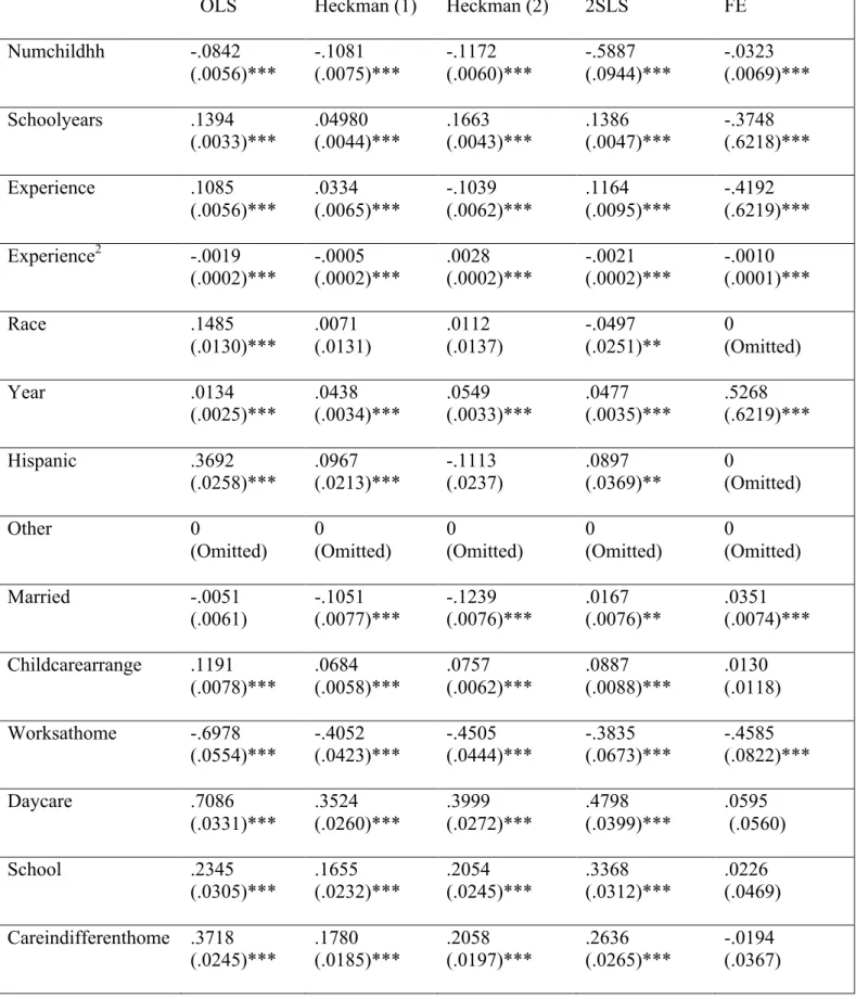
The results for each model are located in the appendix in Table 5, Table 6, and Table 7. Heckman Selection Model for Labor Force Participation
The results for the first Heckman Selection model can be found in Table 5, with the standard errors located beneath the coefficients. The Wald-Chi statistic is 3308.93, which is high, indicating a significance of the whole regression; the Rho estimation of the Heckman model is -.971, indicating the OLS estimates were biased, and that individuals with a higher propensity to work tend to earn a lower wage. The exclusion parameter in the selector equation, the attitude variable on the role of women, is statistically significant, and compared the base answer of strongly disagree, those who disagree, agree and strongly agree are less likely to enter the work force. This indicates that individuals with more traditional values are less likely to choose to enter the workforce. However, those who only agree with the statement are 25% less likely to enter the workforce while those who strongly disagree are 17% less likely to enter the workforce, which doesn’t agree with the trend that those who have more traditional values are more likely to not work.
The second stage of the model indicates that each child an individual has in her
over the years. The coefficient for non-black, non-Hispanic is omitted due to collinearity with the race variable. The geographic location variables indicate that compared to the Northeast, women in all other regions earn less, however the coefficient on the Western region is not statistically significant. In Table 9, the Heckman model was conducted by region, where surprisingly, individuals in the Northeast experienced the largest decrease in wages, and those in the West experienced the smallest, with those in the South had only a 5% decrease. Women who have a higher education attainment level in the south receive a higher wage compared to those with similar schooling in the other regions, with each year of education increasing an individual’s wage by 7%. This infers that those who are college educated is much more valuable in the South, possibly because it may be less common to have job applicants with those credentials. Similarly, those who live in the Northeast or South receive the largest increase in their wages, around 5%, with each additional year of work experience. Those who live in urban areas earn 9.8% more than those who live in rural areas, and when modeled by region, those who live in the West and Northeast benefit the most from living in urbanized locations.
The Childcare variable is positive and statistically significant, indicating that those who have regular childcare for their youngest child, have a 6.8% increase in their wages. Compared to the base of an individual bringing her child to work, the women who have their child watched at home, however the coefficient is small and not statistically significant. Those who use daycare groups, which is normally a paid form of childcare, increase a woman’s wages by 35%.
However, this large increase may be biased due to the fact that individuals who use paid
result possibly indicates that those these individuals may be less efficient since they also have to care for their child.
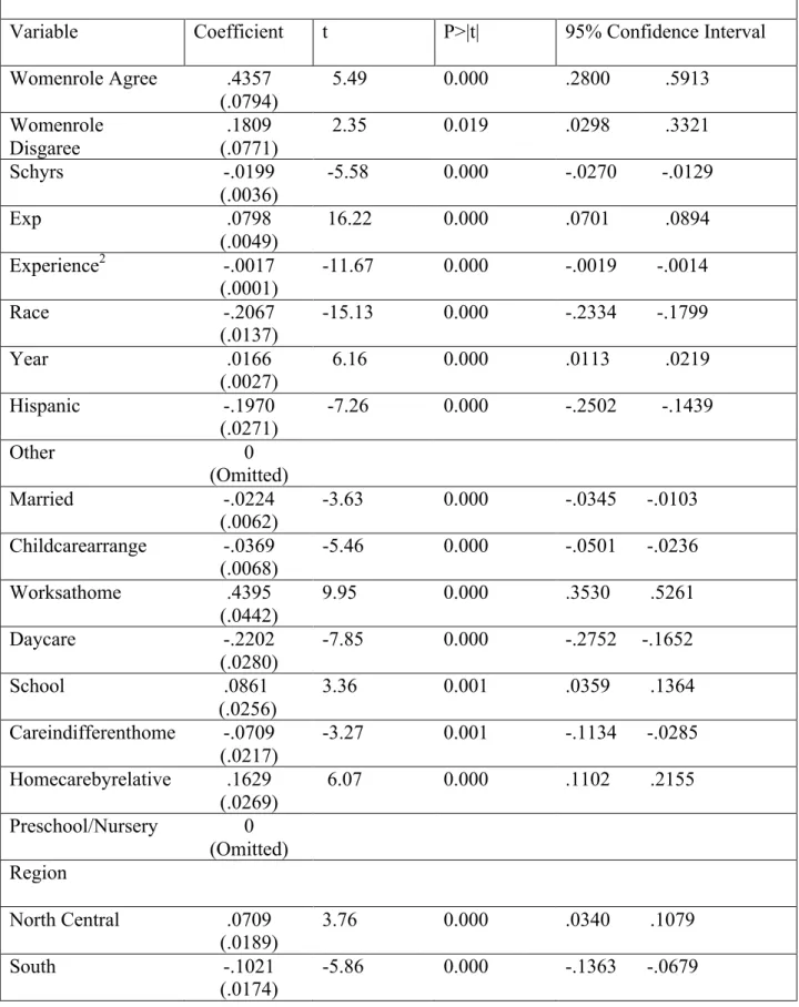
Heckman Selection Model for Motherhood Participation
Similarly, the results for the Heckman Selection model, which can be found in Table 5, for motherhood indicate that the OLS results are biased; the Wald-Chi statistic is 6656.81, which indicates that the entire regression is significant, and the estimation of Rho is -.957, which indicates that the OLS results are biased, meaning those who have the highest propensity to be a mother have the lowest wages, which agrees with expectations. Almost half of the observations are censored; further indicating the original OLS was biased. The exclusion parameter in the selector equation, the attitude variable on an individual’s opinion on traditional roles is statistically significant for the agreement answer compared to the base answer of strongly
disagree, however for those only disagree the coefficient is small and insignificant. Compared to the base answer of strongly disagree, those who strongly agree that traditional roles are best for family are 29% more likely to choose to become a mother. Those who only disagree are only 4% more likely to choose to be a mother.
The second stage of the model yields very similar results to the Heckman model for Labor Force Participation, where each child decreases a woman’s wage by 11.7%; each year of schooling increases wage by 16.6%, which is much larger than the first Heckman model. This model shows that each additional year of work experience negatively affects an individual’s wages, however its squared value is positive, indicating that experience is convex (see figure 2). In this model, those who are categorized as Hispanic actually earn 11% less than black
negative compared to the base answer of Northeast, and those in the Western region have the smallest decrease, while those in the South have the largest decrease, with 12%. Those who live in urban areas see an increase in wages by 10%, which is very similar to the first Heckman model.
The Childcare variable is positive and statistically significant, indicating that those who have regular childcare for their youngest child, have a 7.5% increase in their wages. Similar to the results from the first Heckman model, the childcare options compared to the base of an individual bringing her child to work, the women who have their child watched at home and the women who watch their children while they work experience a negative effect on their wages, however the coefficient on the variable indicating that an individual who has their child watched at home by a relative is not statistically significant. Those who use daycare groups, which is normally a paid form of childcare, increase a woman’s wages by 39%. And both those whose youngest child is in regular school and those whose youngest child is watched in a different residence by a relative see a 20% increase in their wage. Similar to the first model, these results may be biased since only those who use paid forms of childcare are those who already earn higher wages. This is difficult to control and not accounted for in this model. Similarly to the first Heckman Model, individuals who work at home and simultaneously watch their youngest child see a 45% decrease in their wages compared to those who bring their child to work. Two-Stage Least Squares for Reverse Causality
that even though a woman may not hold these traditionally conservative views, she may still choose to have a child. The F-Value of the first stage is 77.89, which is in the range for instrument validity.
The second stage of the model produces statistically significant results, evident by the F-Value of 421.34. Like the previous two models as well as the OLS, the number of children has a significant negative affect on women’s wages, where each additional child in the household decreases wages by 58%, which is a much larger decrease than both OLS and the Heckman models. This large positive relationship may be due to the fact that the instruments indicating an individual’s opinion on family and children may only affect those who feel strongly about the statement. So those who believe that women’s role is in the home, raising children, are much more affected by the instruments, while those who did not necessary have a strong reaction to this statement were not adequately accounted for by the instruments.
Like the previous models, both variables indicating work experience and education indicate a positive increase in wages with and increase in human development. This model also shows that with each additional year, women experience a 4% increase in their wages, which is similar to the other models and past research. When accounting for reverse causality, individuals who are currently or previously married have a small increase in wages compared to those that have not been married, which differs from our other regressions.
Individuals who use any form of childcare for their youngest child also see a 8.8%
increase in their wages compared individuals who bring their children to work, and those that use paid forms of childcare, such as daycare, see a 48% increase in their wages compared to those who bring their youngest child to work. Similar to the results from both Heckman models,
which intuitively makes sense, since these individuals may be less efficient since they may be forced to take more breaks in order to care for their child. Individuals who live in the Southern and North Central regions of the US earn 14% and 10% less than those who live in the
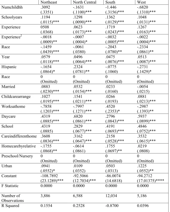
Northeast, and those who live in the Western region only earn 6% less. When evaluating this model by region, which is shown in Table 8 in the appendix, individuals who live in the
Northeast actually experience a positive effect on their wages when they have a child, however this results is not statistically significant. Those who live in the south experience the largest decrease in wages, however this may be due to the fact that the instruments used in the model are only representing individuals who hold these strong beliefs. Individuals in all regions experience a similar increase in their wages with each additional year of education, while women in the South see a 17% increase in their wages with each additional year of work experience, indicating that long-term employment may benefit women more than a large amount of education. Though individuals who live in urban areas do earn more than those in rural areas, the negative impact is half as severe compared to the OLS results; and when modeled by region, those who live in urban areas in the West see a 12% increase in the wages, which is much larger than the increase seen in the Northeast, South, or North Central regions.
Fixed Effects Model
education is negative, which goes against all previous research, however it is not significant at the 5% or 10% level; the effect of increased experience is also negative, which also goes against how work experience normally affects wages. Those who are currently or previously married have 3.5% higher wages than those have never been married, however the coefficient is not statistically significant at the 5% or 10% level, and the results does not largely differ from the coefficient given by OLS.
The use of any form of childcare has a small positive increase of 1.6% on wages,
however this number does largely differentiate from 0 and is much smaller than the results of the other models. Similar to the other models and OLS, individuals who work at home with their children see a 45% decrease in their wages compared to those who bring their child to work. Individuals who have their youngest child watched at home by a spouse or a relative also see a 8% decrease in their wages. All other forms of childcare are positive, however none of them are statistically significant. Individuals who live in the North Central and Southern regions have a -15% and -13% decrease on wages compared to those who live in the Northeast, which is similar to the results in the other models. However, those who live in the West have a -17% decrease in their wages, which is much larger than the results found in all of the other models. After
evaluating this model by region, there was no differentiation in the coefficients on the variable representing the number of children in a household, so the results were not provided in the appendix. Individuals who live in urban have earn 5% more than those who live in rural areas, which is comparable to what the other models produced.
VII. Policy Recommendation
government to provide childcare subsidies. This paper, which is similar to the results of past research, has indicated that each additional child negatively affects wages. This fact combined with the finding that childcare has a positive affect on women’s wages possibly leads to a possible solution for the dilemma that women face when working and being a mother. When controlling for selection bias, care causes a 6% to 11% increase in wages, and when controlling for unobserved heterogeneity, care increases wages by 1.3%. For all models except the Fixed Effects Model, paid childcare, specifically daycare groups, cause a significant increase in wages (see figure 7). Similar results are found for individuals, whose children are in regular school. The theory behind these large increases is that paid childcare like daycare groups and state-funded care, like public schools, provide more reliable, consistent care, which allows mothers to work uninterrupted throughout their day and to possibly work longer hours. A subsidy would allow women from all socioeconomic backgrounds to have access to this service, thus positively affecting their income, as well as reassuring them of the quality of the care.
According to a paper from the Economic Policy Institute, childcare costs account for the greatest variability in family budgets, where monthly childcare costs for a four year old may range from $344 in South Carolina to $1,472 in Washington D.C. For some families, childcare costs may be as high as half of rent in urban areas. Despite women earning more in urban areas, childcare is still expensive and a subsidy would benefit not only families but also firms.
Childcare costs are significantly higher for younger children; and since this paper found that the use childcare for an individual’s youngest child significantly affects their wages, a subsidy would benefit individuals and families (Gould & Cooke, 2015).
subsidies allow for variety of preferences that individuals may have. Though the effect of children on women’s wages vary by state, each additional child negatively affects a woman’s job, which may affect what a mother can provide for her children. By providing a subsidy, a woman can then decide how often and long she prefers to work, as well as how often and how long she prefers to spend time with her child. She also can choose what type of childcare she prefers, allowing for more freedom in consumer choice.
VIII. Conclusion
This paper presents causal evidence that the number children and the use of childcare positively affects women’s wages, and thus overall career earnings. By evaluating panel data over a fifteen-year period of time, and accounting for selection bias, reverse causality, and unobserved heterogeneity in different models, I found that each additional child has a significant negative affect on wages. Childcare has a significant positive effect on wage growth over time, and paid childcare largely increases annual wages. The implications of these results infer that paid childcare, which is often better quality, allow women to focus on their jobs at work, rather than worrying about who is watching their child, thus possibly increasing their productivity.
The paper also evaluated how geographic regions and the urban/rural effect of an
individual’s location has on her wages. Those who live in urban areas have higher wages than those who live in rural areas, which may be due to the larger amount of available jobs as well as the diversity of jobs in urban areas (Figure 4). Corresponding to this finding, individuals who live in the Northeast have higher wages than those who live in the South or the North Central region of the US, especially since the Northeast is historically more urban, with a wider variety of opportunities for their labor force (Figure 5). Both urban areas and the Northeast are
including OLS show that those live in these areas, and thus are less conservative, earn more. This is possibly due to the greater opportunities offered in more urbanized areas, however it is
difficult to tell whether the job opportunities always existed, or that these higher pay jobs were created by the liberal population. This paper focuses on the economic actor as the employee, however these ideological beliefs could affect managers and employers, dictating whom they hire, which would also influence wages. Further research on how ideological beliefs affect hiring patterns would certainly aid these conclusions.
Across all five models, we see a small increase in wages for each additional year, and the negative effect of each additional child, which is similar to the consensus of past literature. The results of the two Heckman Models and 2SLS are significant, and they indicate similar effects on wages. All three models show a negative effect due to the increasing number of children, a positive effect due to childcare use, and a large positive effect that stems from the use of paid childcare compared to an individual to her child to work. All three models use family values as either an exclusion variable or an instrument, and the results, F-values, and Wald-Chi indicate that they are valid, which infers that ideological beliefs affect an individual’s familial choice. The results of the Fixed Effects Model are similar, however, the childcare coefficient is small and not differentiable from zero.
Though all models offer some advantages, the Two-Stage Least Squares provides significant results that are similar to both Heckman models, however almost all of the 2SLS model’s
decrease in wages due to an increase in children, which matches previous literature, however many of the coefficients are statistically significant and since we are not evaluating the consequences of a specific event, the Fixed Effects model may not be the most advantageous model used.
Bibliography
Amuedo-Dorantes, Catalina, and Jean Kimmel, “The Motherhood Wage Gap in the United States: The Importance of Fertility Delay,” Mimeo, 2003.
Angrist, Joshua and William Evans, “Children and Their Parents’ Labor Supply: Evidence from Exogenous Variation in Family Size,” American Economic Review, v. 88 (1998): 450- 477.
Bar, Michael, Seik Kim, and Oksana Leukhina. “Gender Wage Gap Accounting: The Role of Selection Bias.” Demography 52, no. 5 (October 2015): 1729–50. doi:10.1007/s13524-015-0418-x.
Becker, Gary, “Human Capital, Effort, and the Sexual Division of Labor.” Journal of
Labor Economics 3:33-38 (1985).
Blackburn, McKinley, David Bloom and David Neumark, “Fertility Timing, Wage, and Human Capital,” Journal of Population Economics, v. 6 (1993): 1-30.
Budig, Michelle and Paula England, “The Wage Penalty for Motherhood,” American SociologicalReview, v.66 (2001): 204-225.
Bureau of Labor Statistics, “Employment Characteristics of Families-2015,” U.S. Department of Labor, April 2016.
Center on Budget and Policy Priorities, “Policy Basics: The Earned Income Tax Credit,” Center on Budget and Policy Priorities, October 2016.
Chandler, Timothy, Yoshinori Kamo and James Werbel, “Do Delays in Marriage and Childbirth Affect Earnings?” Social Science Quarterly, v. 75 (1994):839-853.
Correll et al., “Getting a Job: Is There a Motherhood Penalty?” American Journal of Sociology, v.112, No. 5 (2007):1297-1339.
Executive Office of the President, October 2014.
Desilver, Drew. “How the Most Ideologically Polarized Americans Live Different Lives.” Pew Research Center, June 13, 2014. http://www.pewresearch.org/fact-tank/2014/06/13/big-
houses-art-museums-and-in-laws-how-the-most-ideologically-polarized-americans-live-different-lives/.
Ellingrud et al., “The Power of Parity: Advancing Women’s Equality in the United States,” McKinsey Global Institute, April 2016.
European Union, “Sweden: Successful Reconciliation of Work and Family Life,” European Platform for Investing in Children, August 2016.
Fuchs, Victor, Women’s Quest for Economic Equality. Harvard University Press, Cambridge: 1988.
Inc, Gallup. “State of the States.” Gallup.com, 2016. http://www.gallup.com/poll/125066/State- States.aspx.
Gould, Elise, and Tanyell Cooke. “High Quality Child Care Is out of Reach for Working Families.” Economic Policy Institute, October 6, 2015.
http://www.epi.org/publication/child-care-affordability/.
Heckman, James J. "Sample Selection Bias as a Specification Error." Econometrica 47, no. 1
(1979): 153-61. doi:10.2307/1912352.
Jacobsen, Joyce and Laurence Levin. 1995. “The Effects of Intermittent Labor Force Attachment on Women’s Earnings.” Monthly Labor Review 118:14-19.
Korenman, Sanders and David Neumark, “Marriage, Motherhood and Wages,” Journal of Human Resources, v. 27 (1992): 233-255