A Reputation-based Distributed District
Scheduling Algorithm for Smart Grids
D. Borra
1,∗, M. Iori
2, C. Borean
2, F. Fagnani
11Dipartimento di Scienze Matematiche, Politecnico di Torino, Italy 2Swarm Joint Open Lab, Telecom Italia, Italy
Abstract
Inthis paperwedevelop and testa distributedalgorithmprovidingEnergy Consumption Schedules(ECS)in
smart grids for a residential district. The goal is to achieve a given aggregate load profile. The NP-hard
constrainedoptimizationproblem reducesto a distributedunconstrainedformulationby meansofLagrangian
Relaxationtechnique,andameta-heuristicalgorithmbasedona QuantuminspiredParticleSwarmwithL´evy
flights. A centralized iterative reputation-reward mechanism is proposed for end-users to cooperate to avoid
power peaks and reduce global overload, based on random distributions simulating human behaviors and
penalties on the effective ECS differing from the suggested ECS. Numerical results show the protocols
effectiveness.
Keywords: DistributedAlgorithms, AutonomousDemand Responsemanagement,EnergyConsumptionScheduling, SmartPowerGrids,Reputationalgorithm
Received on 14 December 2014; accepted on 8 April 2015; published on 28 May 2015
Copyright c 2015 D. Borra et al., licensed to ICST. This is an open access article distributed under the terms of the Creative
Commons Attribution license (http://creativecommons.org/licenses/by/3.0/), which permits unlimited use, distribution and reproduction in any medium so long as the original work is properly cited.
doi:10.4108/cogcom.1.2.e3
1. Intro duct ion
The balance between demand and supply plays a leading role in smart grids applications and modern technologies aim to develop energy optimization algorithms able to provide efficient residential district dispatchment. Distributed optimization methods in power systems play a leading role, due to distributed energy generation and demand, renewables such as photovoltaic resources, storage devices, with changes in real time. A large literature has been devoted to decentralized versions of optimization algorithms applied to power systems, see, e.g., [15], due to distributed energy generation and demand, renewables such as photovoltaic resources, storage devices, with changes in real time. Multi-agent planning, as in [11], is often formulated as a combinatorial optimization problem: each agent has its own objectives, resources, constraints, and at the same time it has to share and compete for global resources and constraints. Moreover, new roles in the energy market are emerging, such as energy aggregators as intermediate between energy utilities and home users,
∗Correspondingauthor.Email:[email protected]
managing uncertanties due to variable customer actions, metereology and electricity prices. Given the huge number of agents, the optimization problem is often computationally intractable in a centralized fashion, and given the time-varying cost and constraints in energy demand-response (DR) problems, a fast single-agent planning algorithm is appealing. In this paper, as in [6], customers are incentivized to move their loads in off-peak hours despite their individual needs through marginal costs, using reputation scores as feedback. In [6] a cooperative game reduces peak-to-average ratio of the aggregate load and the Nash equilibria are reached using centralized information, whereas our approach is completely distributed. Evolutionary Game theory and Reinforcement Learning techniques have been applied to swarm intelligence problems, as in [1, 5,12,14].
Starting from a similar approach, we aim to modify humans behaviors of single houses in the district to follow a given global load curve. Our focus is on energy distribution to a residential district, according to the European Project INTrEPID [9].
In this scenery, the district global load is sensed by power meters, and using non-intrusive load-monitoring techniques (NILM, as in [8]) or smart
plugs, the disaggregated data are available, turning the “blind”system to a decentralized smart grid [2]. A centralized unit senses local loads, and communicates with agents through smart-phone app or similar devices proposing day-ahead optimal Energy Consumption Schedules (ECS). Agents may accept the suggested ECS or not, according to individual needs.
The objectives of our district scheduler are threefold: 1. Following a load profile: act on the system so that
the cumulated district load profile can follow a given load profile;
2. Solving distributed optimization problems: per-form energy optimization of the IoT (Internet of Things) devices (e.g. smart connected appliances) by distributing computational power on different energy boxes (“swarm energy management”); 3. Humans in the loop management: leveraging on
“humans”to “close the loop”for no-IoT devices at home, by providing suggestions to them and tuning the system behavior accordingly.
From a concrete point of view, see the European Project INTrEPID [9], the challenges in the real world are (1) guide cumulated energy consumption for the residential district, (2) schedule smart appliances in a scalable way, and (3) work with the legacy system.
Our contribution is twofold. First, we provide a mathematical formalization of the optimization problem, decoupling the global constraint through Lagrangian relaxation as in [10], see Section 2. Second, in Section
3 we design optimal ECS in a distributed fashion at two levels: at the agent level applying meta heuristic optimization techniques as QPSOL (Quantum Particle Swarm with Levy’s Flights) described in [3], in order to get feasible optimal suggested ECS; at the district level a reputation-reward mechanism provides incentives for users leading to an emerging cooperative behavior. Section 4 describes the numerical results: user habits have been analyzed to simulate user behaviors, based on diffusion of appliances and daily cycles for each appliance. Finally, we draw the conclusions of our study in Section5.
2. Mo del Description
Consider a district withN users, eachi-th agent has ni appliances that are schedulable, like washing machine (WM), dish washer (DW) and tumbler dryer (TD). Refrigerator load is also included as background profile. The state of the multi-agent system is given by x=
(x1, . . . , xN), i.e., a vector of schedules that each user has
to execute daily in a given time slot, and xi is defined by the start times of all theni appliances of useri and their type (WM, DW, TD) with well-known load profiles. More precisely xi∈[0,24]ni and x is the global vector
containing all start times of all users. Due to energy and time constraints, the goal to find a global optimum of the constrained optimization problem, called primal problem:
min x=(x1,...,xN)
N
X
i=1
fi(xi) s.t.
N
X
i=1
gi(xi) =a,
hi(xi)≤bi, i= 1, . . . , N
(1)
where a, bi∈R and the cost function Pifi is a sum of weighted norms of three factors: overload, energy cost and tardiness of the current statex. The first constraint is the only coupling object: gi denotes the peak profile of each user and the global load of the district must attain a given curvea=a(t) depending on time. All the functions fi, gi, hi implicitly depend on time (they span a day), discretized in minutes or hours. The inequalities involving hi are local time and energy (usually 3 kW) constraints of each user. The Lagrange function is
L(x, µ, λi) = N
X
i=1
[fi(xi) +λi(bi−hi(xi))] +µ(gi(xi)−a) (2) whereλi≥0, µare calledLagrange multipliers. Sinceλi can be computed locally, the Lagrange multiplier of our interest isµ, associated to the only coupling constraint. From now on, we neglect the local constraints as they can be included directly in the cost functionsfi. As detailed in [4], the corresponding relaxed dual problem becomes unconstrained:
max
µ x=(xmin1,...,xN)
L(x, µ). (3)
The standard algorithm is as follows: given an initial estimate of µ, each user computes its best ECSx∗i such that
x∗= arg min
x L(x, µ). (4)
Then, x∗ is sent to the central unit, and a subgradient of minxL(x, µ) as function ofµis available. The central unit computes and sends to agents at iteration k:
µ(k)=µ(k−1)+α(k−1) X
i
gi(x∗i)−a
!
, (5)
where α(k−1) is the step length of the gradient descent algorithm. Since the Lagrange multiplier µ can be interpreted as the energy price, in order to decentralize the given dual problem., we split µ=PN
i=1µi. A distributed algorithm that can be applied acts as the previous one with the only difference: agentisolves the optimization problem
min xi
where N gi(xi)−a approximates the global overload
P
jgj(xj)−a. The only computational effort of the central unit is the gradient descent step for µ. The latter optimization problem is solved by means of the population-based metaheuristic method QPSOL, see [3], that reduces a NP-hard combinatorial optimization problem to an adaptive algorithm requiring limited computational power.
Figure 1. The panel displays the communication con-nections in network model, whereas the computation of the optimization problem is distributed among the agents
S1, . . . , SN and the central unit has only to provide a
computationally cheap step of gradient descent, as in Eq. (5).
The underlying idea is to split the optimization algorithm on 2 time scales: (1) the micro-scale concerns the improvement along the day of the day-ahead proposed ECS; (2) the macro-scale involves the reputation-reward mechanisms of the agents, described below, and their collective behavior.
3. Sw arm Simulat or Description
This simulation studies energy distribution to a city district managing its total daily power consumption without power peaks and achieving a given aggregate load curve. Users should follow utility suggestions and receive incentives according to their flexibility. This simulation aims to analyze ways to distribute reward and loads to obtain the best total power curve, considering human behaviors and dynamics. Initially users behave according to some random habits, but they modify their flexibility to perform suggested schedules and asymptotically the multi-agent system stabilizes: in order to encourage users to continue working together, individual credits are spread throughout the possible range. The reward and reputation mechanism explained in what follows aims to give benefits to the most flexible users, in terms of economical awards, e.g. discounts on the flat energy tariffs. Every day users compute local best ECS in a distributed way, according to their needs and utility constraints, as described in Section2. In this Section we focus on the reputation mechanism defining the emerging learning process. Consider best ECS as daily input data. Agents actions define local effective ECS. Two indices evaluate end-users behaviors:
1. reputation depending on start times of effective ECS;
2. reward depending on the distance between best and effective (both local and global) load.
Reputation definition. Each agent may accept or decline ni suggestions, with ni number of appliances. Denote byx∗i the best (sub)-optimal ECS found for Eq.
6 at the end of each day, and denote by ˆxi the effective ECS decided by user i. Formally, the reputation of user ialong the day is
ri = 1−
|x∗i −xˆi| ni
∈[0,1], (7)
, where | · | denotes the distance between the best and effectivei-th ECS in terms of start times of appliances, i.e., reputation decreases as violation rate gets high.
Reward definition. The reward is defined in terms of credits: each agent may earn up to 24 credits each day, comparing hourly the best (b) and effective (e) two quantities: global load and local load. Formally the credits of useriat hourhis defined as
cih= 1−
|glob loadb−glob loade|
glob loadb+ glob loade
−|loc loadb−loc loade|
loc loadb+ loc loade .
(8)
At the end of each day, credits ci∈[0,1] are re-normalized and create rank lists.
Behavior and learning process modeling. Each agent acts based on his own behavior profile, shaped according to
1. favorite start times to schedule appliances; 2. relevance given to reward and reputation by means
of the weight parameter αi∈[0,1], to define reaction to feedback;
3. natural predisposition to follow advice, to set the violation probability, defined by standard deviation σi of a Gaussian distribution.
Best ECS for utility are denoted by the start times vector x∗i and actions are samples from Gaussian distributions
ˆ
xi∼ N(x∗i, σ 2
i), (9)
with mean given by x∗
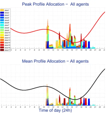
Figure 2. The peak (upper plot) and mean (lower plot) power load (Watts) of a 5 agents neighborhood is displayed at the first of the distributed algorithm proposed in Section 2. The red (black) curve represents the district global load we aim to attain. It has to be compared with the result at the last iteration displayed in Fig.3. All agents are flexible during 10 am-9 pm.
i.e., after each observation period user i evaluates the linear combination of its mean reputation ¯riand its mean reward
¯
ci:qi=αir¯i+ (1−αi)¯ci. (10)
Given the satisfaction threshold (in numerical experiments = 0.6), if qi > , agent i is satisfied and there is a certain probability that relaxes decreasing its standard deviation σi, otherwise it increases according to a fixed discrete random distribution. In conclusion, behavior of agentiis defined by the Gaussian probability density function f =f(x∗i, σi, αi). At each feedback iteration the behavior parameter σi is updated. Houses with best and worse reputations and rewards are listed as another daily feedback, and emerging collective beahvior is described in Section4.2.
4. Numerical Results
4.1. Micro-scale simulation
In this numerical experiments, using MATLAB software we run the simulator for small residential neighborhoods, i.e., N = 5, N = 10 agents and through QPSOL and Lagrangian relaxation described in Section 2, few iterations are sufficient to get a significant reduction of the global overload, as shown in Fig. 2. The output of
Figure 3. The peak (upper plot) and mean (lower plot) power load (Watts) of a 5 agents neighborhood is displayed at the last iteration (t= 10) of the distributed algorithm proposed in Section2. The red (black) curve represents the district global load we aim to attain. All agents are flexible during 10 am-9 pm.
Figure 4. The panel displays the average overload (over 10 samples), i.e., the distance between best and effective global load, as function of algorithm iterations.
such distributed algorithm are the daily suggested ECS, and the macro-scale simulator deals with the learning process acting on human decisions for ECS. In what follows we describe in detail the proposed algorithm on the micro-scale, i.e. performing during the day on the micro-time scale.
• ECS of all users is a vectorx= (x1, . . . , xN);
• Lagrange multipliers, i.e. energy prices of all users µi, i= 1, . . . , N.
Input:
• Cost function f =PN
i=1fi depending on overload, energy cost and tardiness;
• Constraint functions gi, i= 1, . . . , N denoting the peak profile of each user, leading to the global constraint displayed in Eq. (1); constraint function hi, i= 1, . . . , N;
• Global mean load profile a=a(t) and local peak load profile bi=bi(t), i= 1, . . . , N depending on time;
• Gradient descent step α∈(0,1);
At each iteration k:
• Each agent i= 1, . . . , N solve the optimization problem
min
xi fi(xi) +µi(N gi(xi)−a),
by means of a methaeuristic algorithm QPSOL, see [3] for further details;
• Each agent sends its estimatex∗i to the central unit;
• The central unit update the global Lagrange multiplierµas
µ(k)=µ(k−1)+α(k−1) X
i
gi(x∗i)−a
!
,
where α(k−1)=α/(k−1) is the gradient descent step, decreasing as the iteration is large. Then, the central unit updates the local energy prices, i.e. Lagrande multipliers such that P
iµi=µ, as follows
µ(k)i =F(µ(k), x∗i)
where F is a function decreasing with the load of agent i with ECS x∗i. An example for F is a line F(µ(k)) = 1−µ(k), whereµ(k)actually depends on x∗i.
Output:
• Each agent knows its daily optimal ECS x∗
i(∞);
• The central unit knows the final Lagrange mul-tipliers µi(∞) and the approximated global opti-mal state x∗(∞) = (x∗1(∞), . . . , x∗N(∞)) solving the NP-had constrained optimization problem dis-played in Eq. (1).
Figure 5. The upper plot shows the maximum (blue) and minimum (red) difference in percentage (converging to 20%) between best and effective total load varying the number of houses from 15 to 500. The plot below refers to necessary time to the district to reach a stable state (3−6 months) and a stable difference between the two loads, compared to the number of houses from15to500.
4.2. Macro-scale simulation
Software used for the development of macro-scale simulation is GAMA-platform [7], an agent-based, spatially explicit, modeling and simulation platform. Models are written in the GAML agent-oriented language, so that each house is considered to be an agent. We consider a district composed by N = 100 houses and a scheduled annual load for each resident about 1200−1400kW h.
Each agent at the beginning of the day will decide which and how many appliances would like to program. All houses compute the best load profile and decide to follow it or not. At the end of this process they send to central unit their data so that it can assess their behavior and spread credits.
use every appliance no more than once a day, 50% no more than twice and 10% no more than three times a day. Some exceptions are considered. Some users have also the ability to generate energy with solar panels, but they cannot share it with their neighbors.
Each agent acts based on his own behavior profile. This is shaped according to user reaction to the following different topics:
• Favorite times to schedule appliances: three time areas are identified as favorite and are shared with different probability. These regions are late afternoon, early morning and middle hours of the day.
• Relevance given to reward and reputation:agents can perceive feedback in several ways, in particular someone could give more importance to reputation, someone else to reward and other one could consider equally significant these two parameters.
Figure 6. The charts are two examples of the values assumed by the total effective load (red) and the total best load (green) in the different hours of the day. The plot on the left represents the situation when the simulation starts, while in the right one the situation is stabilized.
• Natural predisposition to follow advice: there are three possibilities also in this case and agents are splint according on their tendency to take an active part in the multi-agent distributed system. Some users are interested in satisfy utility demands, other instead prefer not to schedule their appliances and finally some other try to balance these two trends.
Profiles are spread according to certain probability distributions and there is a little probability that agents change a specific profile during simulation. Moreover this classification is not so hard and some exceptions are taken into account.
Every day agents receive suggestions on load coming from the central unit and they are rewarded based
on how they follow these advices. The purpose of the implemented optimization is to reduce the difference between the cumulative effective ECS and the cumulative best one. During simulation users learn to follow suggestions, in line with their behavior profile. The learning process depends on relevance that they give to reward and reputation. If they decide to not take the advice, they will schedule appliances in their “favorite times”.
The energy utility awards prizes according on behaviour of agents and on credits that each user obtained in a fixed period. During the day time each agent can gain a maximum of 24 credits, one for hour. At any time, credits depends both on individual behavior and cumulative conduct. Rewards are redistributed according to rank list to encourage users to continue working together and following advice. Who does not consider the suggestions is doubly penalized, while virtuous people are rewarded even further. In this way concentrations of agents with the same score are avoided. Agent reputation is defined by rate of advice violation and run in range [0,1]. Violation rate changes depending
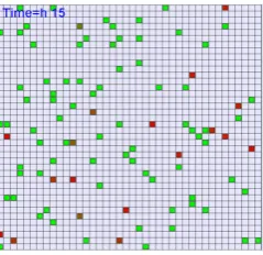
Figure 7. The picture displays houses in a district using the software Gama. The red houses are the ones with effective ECS slightly different from the suggested ECS, whereas the green houses are the more reliable and energy efficient. The used software allows a dynamic visualization as the iterations of the algorithm run.
on how they move from suggestion and increases with the hours difference between appliance best scheduling and effective scheduling.
Residents received periodic feedback on their conduct:
• Mean reputation in these days (from the previous feedback) in relation to best reputation. In fact reputation is a parameter for comparison with the other agents.
• Mean reward obtained in these days.
values of violation and reward and so system finds a balance, after a lot of days.
The system evolution stabilizes in the presence of perturbative phenomena on the input parameters, i.e., differences between effective and best ECS. Using default value of parameters we can reach a mean percentage difference (over the best load) between the best total load and the effective total load converges to 20% as in Fig.5(upper plot).
Varying the number of houses, the difference between effective and best load profile stabilizes starting from 100 houses in the district, as shown in Fig. 5 (the bottom chart). From numerical simulations with our setting (N = 100 houses), convergence time varies between 3 and 6 months. Reported values are the average over 10 simulations with the same numberN of homes. Variance is greater if we consider few houses, while stabilization time increases withN.
In what follows, we describe in detail the algorithm iterations we propose on the macro-scale, i.e. perfoming along days and stabilizing after weeks or months.
Input:
• The number of appliances of each agent ni, i= 1, . . . , N;
• The initial reputation of each agent ri∈[0,1], i= 1, . . . , N;
• The initial reward of each agent i for every time slot (hour) h, i.e. cih∈ {0,1}, i= 1, . . . , N, h= 1, . . . ,24;
• Weight parameter αi∈[0,1] that is the relevance each agent gives to reward and reputation to define its reaction to feedback,
• Standard deviation σi, i= 1, . . . , N for Gaussian distribution N(0, σi) modeling predisposition to follow advice. Such value is initially sampled from a Uniform distribution in a preset rangeσi∈[σ1, σ2];
• Behavior satisfaction threshold (in numerical experiments we choose e.g. = 0.6). It is a weight that defines a tradeoff between the reputation and the reward, thus it is a real value in (0,1). For any other value in (0,1) there is no significant change in the results.
At each day/iteration k:
• Each agent decides how many appliances to program, between 1 and ni;
• Each agent computes the best load profile based on the suggestions received from utility x∗i(k) (see micro-scale algorithm);
• Each agent decides to follows the suggestion or not, performing the effective schedule ˆx(k)i . Its decision
is based on its behavior characteristics: ˆ
x(k)i ∼ N(x∗i(k), σi)
• reputation and rewards are updated and are given to agents as feedback
r(k)i = 1−|x
∗(k) i −xˆ
(k) i | ni
∈[0,1]
c(k)ih = 1−|glob loadb−glob loade|
glob loadb+ glob loade
−|loc loadb−loc loade|
loc loadb+ loc loade .
and the total credits can be at most 24 and then they are normalized in [0,1], defined as ¯ci=
P
hcih/|Phcih|;
• each agent reacts evaluating q(k)i =αir¯
(k)
i + (1−αi)¯c (k) i .
Ifqi> , agentiis satisfied and relaxes decreasing
its standard deviationσi(k), otherwise it increases, i.e.
σ(k)i =F(σi(k−1), q(k)i ). Output:
• Asymptotic rewards and reputations
¯
ci(∞), ri(∞), i= 1, . . . , N;
• Global load attained by the residential district depending on effective schedules ECS xˆ =
(ˆx1, . . . ,xˆN), approaching the optimal suggested
ECSx∗= (x∗1, . . . , x∗N).
5. Conclusions
In this paper we provide a mathematical model and a simulator of an energy distribution system applied to a residential district. Once end-users compute local optima in a distributed way, human decisions are modeled and a reputation-reward mechanism is performed on large numbers. Numerical results prove the efficiency of our algorithm: on the macroscale with few houses (150) the difference between best and effective ECS converges to 20%, and with an average time of 3 months the district stabilizes. Moreover, the approach will be verified on the field with real devices and application in the INTrEPID project pilot.
extended model we are going to study aims to to recover who is not cooperative: few residents, who are not usual to comply with the advice, are free to plan their load as they prefer, but they will have penalties in place of awards. On the contrary, the rest of users will have to compensate for the total load receiving a higher reward. This more adaptive system aims to attain the global load curve more precisely, considering and involving agents habits and schedules predictions.
Acknowledgments. Authours would like to thank Ennio Grasso for the scientific hints on the mathematical modeling and numerical implementation. The project has been partly funded by INTrEPID EU FP 7 project [9], grant n. 317983.
References
[1] Baharlouei, Z.; Hashemi, M.; Narimani, H.; Mohsenian-Rad, H.: Achieving optimality and fairness in autonomous demand response: benchmarks and billing mechanisms, IEEE Transactions on Smart Grid, 4(2), pp.968–975, (2013)
[2] Borean, C.; Ricci, A.; Merlonghi, G.: Energyhome: a user-centric energy management system, Metering International 3, pp. 52, (2011)
[3] Borean, C.; Grasso, E.: QPSOL: quantum particle swarm optimization with Levys flight, ICCGI 2014, Seville, Spain, (2014)
[4] Boyd, S.; Vandenberghe, L.: Convex optimization, Cambridge University Press, (2004)
[5] Campos-Nanez, E.; Garcia, A.; Li, C.: A game-theoretic approach to efficient power management in sensor networks, Operat. Res., 56(3), pp. 552, (2008)
[6] Caron, S.; Kesidis, G.: Incentive-based energy consump-tion scheduling algorithms for the smart grid, IEEE International Conference on Smart Grid Communica-tions (SmartGridComm), pp.391–396, (2010)
[7] GAMA-platform, https://code.google.com/p/ gama-platform/
[8] Hart, G. W.: Nonintrusive appliance load monitoring, Proceedings of the IEEE 80 (12): 1870, (1992)
[9] INTrEPID, FP7-ICT project, http://www. fp7-intrepid.eu/
[10] Jhi-Young Joo; Ilic, M.D.: Multi-layered optimization of demand resources using Lagrange dual decomposition, IEEE Transactions on Smart Grid, 4(4), pp.2081–2088, (2013)
[11] Krause, J., et al.: A survey of swarm algorithms applied to discrete optimization problems, Swarm Intelligence and Bio-inspired Computation: Theory and Applications. Elsevier Science & Technology Books, pp. 169–191, (2013)
[12] Liyan J.; Lang T.: Day ahead dynamic pricing for demand response in dynamic environments, IEEE Conference on Decision and Control (CDC), pp. 5608– 5613, (2013)
[13] Pinyol, I.; Sabater-Mir, J.: Computational trust and reputation models for open multi-agent systems: a review, Artificial Intelligence Review, 40(1), pp. 1–25 (2013)
[14] Tuyls, K.; Nowe, A.: Evolutionary game theory and multi-agent reinforcement learning, The Knowledge Engineering Review, 20(01), pp. 63-90, (2005)