Investigating the impact of simple and mixture priors on estimating sensitive proportion through a general class of randomized response models

(1)

Sharif University of Technology

Scientia Iranica

Transactions E: Industrial Engineering http://scientiairanica.sharif.edu

Investigating the impact of simple and mixture priors

on estimating sensitive proportion through a general

class of randomized response models

M. Abid

a,b,*

_{, A. Naeem}

c

_{, Z. Hussain}

d

_{, M. Riaz}

e

_{, and M. Tahir}

a a. Department of Statistics, Government College University, Faisalabad, 38000, Pakistan.

b. Department of Mathematics, Institute of Statistics, Zhejiang University, Hangzhou, 310027, China. c. Government Degree College for Women, Samanabad, Faisalabad, 38000, Pakistan.

d. Department of Statistics, Quaid-i-Azam University, Islamabad, 44000, Pakistan.

e. Department of Mathematics and Statistics, King Fahad University of Petroleum and Minerals, Dhahran, 31261, Saudi Arabia. Received 14 June 2017; received in revised form 12 December 2017; accepted 27 June 2018

KEYWORDS Bayesian estimation; General randomized response model; Loss functions; Population proportion; Prior distributions.

Abstract. Randomized response is an eective survey method to collect subtle information. It facilitates responding to over-sensitive issues and defensive questions (such as criminal behavior, gambling habits, drug addictions, abortions, etc.) while maintaining condentiality. In this paper, we conducted a Bayesian analysis of a general class of randomized response models by using dierent prior distributions, such as Beta, Uniform, Jereys, and Haldane, under squared error loss, and precautionary and DeGroot loss functions. We have also expanded our proposal to the case of mixture of Beta priors under squared error loss function. The performance of the Bayes and maximum likelihood estimators has been evaluated in terms of mean squared errors. Moreover, an application with real dataset has been also provided to explain the proposal for practical considerations. © 2019 Sharif University of Technology. All rights reserved.

1. Introduction

Sample surveys on human population have come to a realization that innocent and inoensive questions usually receive good responses, whereas questions about delicate and sensitive matters involving defensive contentions and controversial assertions, stigmatizing and/or incriminating matters (such as induced abor-tion, tax evasion, cheating at the exams, drug usage, illicit behaviors, etc.), which people like to conceal from *. Corresponding author. Tel.: 0092 3336289936

E-mail addresses: mhmmd [email protected] (M. Abid); [email protected] (A. Naeem);

[email protected] (Z. Hussain);

[email protected] (M. Riaz); [email protected] (M. Tahir).

doi: 10.24200/sci.2018.20166

others, elicit reluctance. Attempting to ask questions such matters often results in either negation to respond, or deception in answering. This introduces non-response error that makes the estimation of relevant parameters, e.g., population proportion belonging to a sensitive group, unreliable.

To abolish this problematic issue of unresponsive-ness or non-response, Warner introduced an ingenious interviewing procedure, known as the Randomized Re-sponse Technique (RRT), for stimulating information about subtle and sensitive characteristics [1]. The main aim of Warner [1] RRT was to reduce the frequency of distorted (misleading) answers, increase respondents' cooperation, and obtain truthful responses by asking respondents two questions, one of which is sensitive and the other is non-sensitive. By means of a randomization device (such as drawing a card from deck, rolling a die, spinning a roulette wheel, etc.), the respondents choose

(2)

one of the two questions. It makes the interviewees less likely to give an imprecise answer. Several researches, such as Greenberg et al. [2], Moors [3], Kim et al. [4], Christodes [5], Hussain and Shabbir [6], Kim and Heo [7], Lee et al. [8], Abdelfatah and Mazloum [9], Tanveer and Singh [10], Blair et al. [11], and Singh and Gorey [12], contributed to further development of the RRT model. The interested readers may also refer to Chaudhuri and Mukerjee [13], Tracy and Mangat [14], Chaudhuri [15], Chaudhuri and Chirstodes [16], and the references listed therein.

Estimation of the unknown parameter (s) is car-ried out after collecting the data through RRT. For the estimation of unknown parameter(s), two familiar methods are mainly used: the classical method and the Bayesian method. The Bayesian method can be useful in a situation when the prior knowledge about the perceptive qualitative variable is generally available in a social survey and can be used besides sample information for estimating the unknown population pa-rameters. In addition, the Bayesian technique provides a normal way to study and deduce situations such as randomized response sampling where only limited in-formation is available. Although the Bayesian analysis of RRTs has been studied, only a few attempts have been made in this area, e.g., Winkler and Franklin [17], Migon and Tachibana [18], Pitz [19], O'Hagan [20], Spurrier and Padgett [21], Oh [22], Unnikrishnan and Kunte [23], Barabesi and Marcheselli [24,25], Hussain and Shabbir [26-28], Hussain et al. [29], and Bar-Lev et al. [30].

Winkler and Franklin [17] rst suggested the RRT in the framework of Bayesian structure by using Beta distribution as the prior distribution. Bar-Lev et al. [30] performed the Bayesian analysis of the RRT, considering the truncated Beta prior distribu-tions. O'Hagan [20] derived Bayes linear estimators by utilizing the nonparametric approach. Oh [22] and Un-nikrishnan and Kunte [23] utilized Markov chain and Monte Carlo approaches, respectively. Adepetun and Adewara [31] conducted Bayesian estimation of Kim and Warde RRT based on alternative priors. Hussain et al. [32] performed a Bayesian analysis of a general class of RRTs using a simple Beta prior in a common prior structure to obtain the Bayesian estimation of the proportion of stigmatized/sensitive attributes in the population of interest and also extended their proposal to stratied random sampling. Son and Kim [33] performed the Bayesian analysis of two-stage and stratied RRTs. Song and Kim [34] proposed the Bayes estimator of a rare attribute using RRT, and showed that their Bayes estimator was robust to priors. Now, by considering the Winkler and Franklin's [17] idea of identifying prior information and analyzing the posterior distribution (as done by Hussain et al. [32]), we proposed to study a general

class of RRTs yielding and eliciting the probability of a yes response given as follows:

P (yes) = = cA+ g; (1)

where c and g are RRT-dependent real numbers, A is the true, yet known, population proportion of

individuals with sensitive traits.

The probability of a yes response through Warner's [1] randomized response model can be written as follows:

P (yes) = = (2p 1)A+ (1 p): (2)

Therefore, by comparing Eq. (1) with Eq. (2) values of c and g are obtained as follows:

c = (2p 1); g = (1 p):

Therefore, we can see that the general class of RRT can be reduced to Warner [1] model, if we consider c = (2p 1) and g = (1 p).

On the same lines, the general class of RRT can be converted to other randomized response techniques.

Now, from Eq. (1), we have: A= g_c ; 0 < A< 1:

The Maximum Likelihood Estimator (MLE) of A is

specied as follows:

^A(ML)= ^ g_c ; (3)

where ^ = n1

n is the sample proportion of yes responses

in a sample of size n.

In this study, we plan to perform the Bayesian estimation of a general class of RRT by using several prior distributions (such as Beta, Uniform, Jereys and Haldane) under dierent loss functions (such as squared error, precautionary and DeGroot). The main purpose of this study is to identify which prior distribu-tions perform better under which loss function, because a situation may arise when dierent researchers have dierent prior beliefs. The Bayesian estimation of general class of RRT by using mixture prior is also performed in this study.

The rest of the paper is structured as follows. Sec-tion 2 presents the details of loss funcSec-tions. Bayesian estimation of a general class of RRT in case of dierent priors under dierent loss functions is presented in Section 3. Section 4 contains the eciency compar-isons. Illustration of the procedure using real dataset is evaluated in Section 5. Final remarks and conclusion are provided in Section 6.

2. Loss functions

A loss function shows losses incurred when estimating parameter by ^. Many loss functions have been-proposed to perform Bayesian estimation. This study

(3)

considers the three loss functions, described below. 2.1. Squared error loss function

Legendre [35] and Guass [36] used the Squared Error Loss Function (SELF) to develop least square theory. Afterwards, it was used in estimation problems when unbiased estimators of parameter were evaluated in terms of the risk function, which was simply the variance of the estimators. The SELF can be expressed as follows:

LSELF(^; ) = ( ^)2:

The Bayes estimator under SELF can be obtained as follows: ^Bayes= E(=x)():

2.2. Precautionary loss function

Norstrom [37] proposed an alternative asymmetric Precautionary Loss Function (PLF), and showed that his proposed PLF was a special form of a general class of precautionary loss functions. The PLF is dened as follows:

LPLF(^; ) = ( ^) 2

^ :

The Bayes estimator under PLF can be written as follows: ^Bayes=pE(=x)(2).

2.3. DeGroot loss function

DeGroot [38] introduced dierent types of loss func-tions and found Bayes estimates by using these loss functions. If ^ is an estimate of ; then, by using the data Xn _{= (X}

1; X2; :::; Xn), the DeGroot Loss

Function (DLF) is given as follows: LDLF(^; ) = ( ^)

2

^2 :

The Bayes estimator under DLF can be derived by using the following formula:

^Bayes=E(=x)( 2₎

E(=x)():

3. Bayesian estimation of A using general

randomized response model

To obtain Bayesian estimator of A, dierent prior

distributions (such as Beta, Uniform, Jereys and Hal-dane) under dierent loss functions (such as squared error, precautionary and DeGroot) are used. These priors are selected according to the range of the parameter, i.e., 0 < A < 1. Using these prior

distributions and loss functions, the Bayes estimators of Aare obtained as follows.

3.1. Posterior distribution and Bayes estimators of A using beta prior

The rst prior distribution considered in this study is

the Beta prior. There are two main reasons for using the Beta prior. The rst one is that Beta prior is a conjugate prior distribution for the Bernoulli, binomial, negative binomial and geometric distributions. The second is that the Beta prior is a suitable prior for the random behavior of percentages and proportions. Of note, with Beta prior, we have a closed-form expression of the Bayes estimator.

Let prior distribution of Abe given by:

f(A) =_{(a; b)}1 a 1A (1 A)b 1;

0 < A< 1 and a; b > 0;

where a and b are the hyper parameters. Let T = Pn

i=1xi be the total number of yes

re-sponses in a sample of size n drawn from the population using simple random sampling with replacement (SR-SWOR). Herein, xi = 1 and xi = 0 with probabilities

of and (1 ), respectively.

Therefore, the conditional distribution of T known as A is written as follows:

f(T=A) =_{t!(n t)!}n! t(1 )n t: (4)

Putting Eq. (1) into Eq. (4), we have: f(T=A) = n!c

n

t!(n t)!(A+ d)t(1 A+ h)n t; where t = 0; 1; 2; :::; n, d = g_c and h = 1 c g_c .

After some algebraic work, we get: f(T=A) = n!c

n

t!(n t)!

t

X

i=0 n t

X

j=0

(n t)! j!(n t j)! t!

i!(t i)!dt ihn t jiA(1 A)j:

The joint distribution of T and Ais written as follows:

f(T; A) = n!c n

t!(n t)!(a; b)

t

X

i=0 n t

X

j=0

(n t)! j!(n t j)!

t!

i!(t i)!dt ihn t ja+i 1A

(1 A)b+j 1:

The marginal distribution of T is obtained by in-tegrating the joint distribution of f(T; A) into A.

Therefore, the marginal distribution of T is: f(T ) = _{t!(n t)!(a; b)}n!cn

t

X

i=0 n t

X

j=0

(n t)! j!(n t j)! t!

(4)

f(A=T ) = f(T; _{f(T )}A); f(A=T ) = t

P

i=0 n t_P j=0

(n t)!

j!(n t j)!i!(t i)!t! dt ihn t jAa+i 1(1 A)b+j 1 t

P

i=0 n t_P j=0

(n t)!

j!(n t j)!i!(t i)!t! dt ihn t j(a + i; b + j)

(0 < A< 1):

(5) Box I

^A(Bayes)Beta= t

P

i=0 n t_P j=0

(n t)!

j!(n t j)!i!(t i)!t! dt ihn t j(a + i + 1; b + j) t

P

i=0 n t_P j=0

(n t)!

: (6)

Box II Posterior distribution of A given T is dened by

Eq. (5) as shown in Box I. The Bayes estimators using the Beta prior under the dierent loss functions, such as SELF, PLF, and DLF, are given as follows: Bayes estimator of Ausing Beta prior under SELF

is obtained by Eq. (6) as shown in Box II, similarly: Bayes estimator of A using Beta prior under PLF

is obtained by Eq. (7) as shown in Box III.

Bayes estimator of A using Beta prior under DLF

is obtained by Eq. (8) as shown in Box IV. 3.2. Posterior distribution and Bayes

estimators of A using Uniform prior

When the prior distribution has no population basis, it can be dicult to construct, and there has long been a

desire for a prior distribution that can be guaranteed to play a minimal role in the posterior distribution. Such distributions are sometimes called as \reference prior distributions", and the prior density is described as vague, at, defuse or non-informative prior. The rationale or using non-informative prior distributions is said to be: \let the data speak for themselves"; therefore, the inferences are unaected by information external to the current data. There are dierent informative priors, yet we have used the non-informative Uniform prior in this study given as follows.

f(A) / 1; 0 < A< 1:

The posterior distribution using Uniform prior is written as follows:

^A(Bayes)Beta=

v u u u u u u t

t

P

i=0 n t_P j=0

(n t)!

P

i=0 n t_P j=0

(n t)!

: (7)

Box III

^A(Bayes)Beta= t

P

i=0 n t_P j=0

(n t)!

P

i=0 n t_P j=0

(n t)!

j!(n t j)!i!(t i)!t! dt ihn t j(a + i + 1; b + j)

: (8)

(5)

f(A=T )

=

t

P

i=0 n t_P j=0

(n t)!

j!(n t j)!i!(t i)!t! dt ihn t jiA(1 A)j t

P

i=0 n t_P j=0

(n t)!

j!(n t j)!i!(t i)!t! dt ihn t j(i+1; j+1)

;

0 < A< 1: (9)

The Bayes estimators of A under dierent loss

functions by using the non-informative Uniform prior can be obtained as follows.

Bayes estimator of A using Uniform prior under

SELF is obtained as followes: ^A(Bayes)Uniform

=

t

P

i=0 n t_P j=0

(n t)!

j!(n t j)!i!(t i)!t! dt ihn t j(i + 2; j + 1) t

P

i=0 n t_P j=0

(n t)!

j!(n t j)!i!(t i)!t! dt ihn t j(i + 1; j + 1)

: Bayes estimator of A using Uniform prior under

PLF is obtained as followes: ^A(Bayes)Uniform=

t

P

i=0 n t_P j=0

(n t)!

P

i=0 n t_P j=0

(n t)!

:

Bayes estimator of A using Uniform prior under

DLF is obtained as followes: ^A(Bayes)Uniform=

t

P

i=0 n t_P j=0

(n t)!

P

i=0 n t_P j=0

(n t)!

: 3.3. Posterior distribution and Bayes

estimators of A using Jereys' prior

Another non-informative prior used to nd Bayes

estimator of A is Jereys' prior. Jereys' prior is

widely used in Bayesian analysis. Jereys' priors can work well in the case of a single parameter model, but not for models with multidimensional parameter vector. It is dened as follows:

f(A) / A1=2(1 A) 1=2; 0 < A< 1:

The posterior distribution of A using Jereys'

prior is given as follows: f(A=T ) =

t

P

i=0 n t_P j=0

(n t)!

j!(n t j)!i!(t i)!t! dt ihn t ji 0:5A (1 A)j 0:5 t

P

i=0 n t_P j=0

(n t)!

j!(n t j)!i!(t i)!t! dt ihn t j(i + 0:5; j + 0:5)

;

0 < A< 1: (10)

Now, the Bayes estimators of A using Jereys' prior

under dierent loss functions are given as follows: Bayes estimator of A using Jereys' prior under

SELF

^A(Bayes)Jereys= t

P

i=0 n t_P j=0

(n t)!

j!(n t j)!i!(t i)!t! dt ihn t j(i+1:5; j+0:5) t

P

i=0 n t_P j=0

(n t)!

j!(n t j)!i!(t i)!t! dt ihn t j(i+0:5; j+0:5)

: Bayes estimator of A using Jereys' prior under

PLF is obtained as shown in Box V.

Bayes estimator of A using Jereys' prior under

DLF is obtained as shown in Box VI. 3.4. Posterior distribution and Bayes

estimators of A using Haldane prior

The last prior considered in this study is the Haldane prior. The Haldane prior can be written as follows:

f(A) / 1

A(1 A); 0 < A< 1:

Of note, the Haldane prior is an improper prior, because its integration (from 0 to 1) fails to converge to 1.

^A(Bayes)Jereys=

v u u u u u u t t P i=0 n t_P j=0

(n t)!

j!(n t j)!i!(t i)!t! dt ihn t j(i + 2:5; j + 0:5) t

P

i=0 n t_P j=0

(n t)!

j!(n t j)!i!(t i)!t! dt ihn t j(i + 0:5; j + 0:5)

:

(6)

^A(Bayes)Jereys== t

P

i=0 n t_P j=0

(n t)!

j!(n t j)!i!(t i)!t! dt ihn t j(i+2:5;+j+0:5) t

P

i=0 n t_P j=0

(n t)!

j!(n t j)!i!(t i)!t! dt ihn t j(i+1:5; j+0:5)

:

Box VI The posterior distribution of Agiven T using the

Haldane prior is given as follows: f(A=T ) =

t

P

i=0 n t_P j=0

(n t)!

j!(n t j)!i!(t i)!t! dt ihn t jAi 1(1 A)j 1 t

P

i=0 n t_P j=0

(n t)!

j!(n t j)!i!(t i)!t! dt ihn t j(i; j)

;

0 < A< 1: (11)

The Bayes estimators of Ausing Haldane prior under

dierent loss functions are given as follows:

Bayes estimator of A using Haldane prior under

SELF is obtained as followes: ^A(Bayes)Haldane

=

t

P

i=0 n t_P j=0

(n t)!

j!(n t j)!i!(t i)!t! dt ihn t j(i + 1; j) t

P

i=0 n t_P j=0

(n t)!

: Bayes estimator of A using Haldane prior under

PLF is obtained as shown in Box V. ^A(Bayes)Haldane=

v u u u u u u t t P i=0 n t_P j=0

(n t)!

P

i=0 n t_P j=0

(n t)!

: Bayes estimator of A using Haldane prior under

DLF ^A(Bayes)Haldane = t P i=0 n t_P j=0

(n t)!

P

i=0 n t_P j=0

(n t)!

j!(n t j)!i!(t i)!t! dt ihn t j(i + 1; j)

: 3.5. Posterior distribution and Bayes

estimators of A using mixture prior

The use of mixtures as prior distributions allows for

greater exibility in the shape of the prior density. The mixture prior is helpful in situations when dierent researchers have their dierent views about the shape of the distribution of the parameter of interest.

Let us assume that there will be participa-tion of K researchers by their specic views about the prior distribution, and these are indicated by f1(A) ; f2(A) ; :::; fK(A). A mixture of prior

dis-tributions can be dened as follows: f (A) =

K

X

k=1

wkfk(A);

where w1; w2; w3; :::::; wk are the weights, such that K

P

k=1wk= 1. Thus, the belief of the kth researcher in

the form of Beta density as a prior distribution can be written as follows:

fk(A=ak; bk) =_(a1 k; bk)

ak 1

A (1 A)bk 1;

0 A 1: (12)

Therefore, the mixture of priors is given as follows: f(A=a0s; b0s) =

K

X

k=1

wk_(a1 k; bk)

ak 1

A (1 A)bk 1;

0 A 1; (13)

where a1; a2; a3; :::; aK and b1; b2; b3; :::; bK are the

pa-rameters of component Beta distribution.

By using Eq. (13), the conditional distribution of T given A is specied as follows:

f(T=A) = n!c n t!(n t)! K X k=1 wk

(ak; bk) t X i=0 n t X j=0 t! i!(t i)! (n t)!

j!(n t j)!dt ihn t j(ak+i; bk+j)

; (14) where t = 0; 1; 2; :::; n, d =g_c and h = 1 c g_c .

Hence, the posterior distribution is calculated by Eq. (15) as shown in Box VII. Now, the Bayes estimators using mixture prior under SELF in the closed form are given by Eq. (16) as shown in Box VIII.

(7)

f(A=T ) = K

P

k=1

wk

(ak;bk)

t

P

i=0 n t_P j=0

t!

i!(t i)!j!(n t j)!(n t)! dt ihn t jAak+i 1(1 A)bk+j 1

K

P

k=1

wk

(ak;bk)

t

P

i=0 n t_P j=0

t!

i!(t i)!j!(n t j)!(n t)! dt ihn t j(ak+ i; bk+ j)

(15)

Box VII

^A(Bayes)mixture= K

P

k=1

wk

(ak;bk)

(

t

P

i=0 n t_P j=0

t!

i!(t i)!j!(n t j)!(n t)! dt ihn t j(ak+ i + 1; bk+ j)

)

K

P

k=1

wk

(ak;bk)

(

t

P

i=0 n t_P j=0

t!

i!(t i)!j!(n t j)!(n t)! dt ihn t j (ak+ i; bk+ j)

) (16)

Box VIII 4. Eciency comparisons and discussion

According to Eqs. (6), (7), and (8), the Bayesian estimator involves a large computation, especially when the sample size and/or the number of yes responses is large. To deal with this computational issue, we have written a program in R and Mathematica software.

Of note, the study of the posterior distribution can provide a picture of the inuence of sample infor-mation on the prior estimate. Therefore, the posterior means and variances using the posterior distributions dened in Eqs. (5), (9), (10), and (11) for all the selected priors are given in Tables 1-3 under all the loss functions considered in this study.

Once a Bayes estimator is calculated, the next task is to compare Bayes estimator with its

com-peting estimators (e.g., the MLEs). It is obvious that the description of posterior distribution does not support the comparison of the Bayes estimator with the classical estimator. These two estimators may be compared in terms of either variance and/or the Mean Squared Error (MSE). Therefore, to compare the Bayes estimator with the classical estimator in terms of MSE, we adopt the approach suggested by Chaubey and Li [39].

4.1. Bayes estimators of simple prior versus MLE

Now, the MSEs of dierent estimators in Bayesian and classical settings, with simple priors (such as Beta, Uniform, Jereys and Haldane) and mixture priors

Table 1. Description of posterior distribution for dierent loss functions for n = 10, and t = 4.

Loss function c g Beta (5, 10) Beta (12, 16) Uniform Jereys Haldane

Mean Variance Mean Variance Mean Variance Mean Variance Mean Variance Squared error

loss function 0.1

0.1 0.365 0.014 0.446 0.008 0.649 0.065 0.715 0.085 0.887 0.099 0.3 0.382 0.013 0.452 0.008 0.666 0.053 0.739 0.064 0.957 0.040 0.5 0.374 0.012 0.444 0.007 0.581 0.050 0.625 0.069 0.909 0.082

Precautionary loss function 0.1

0.1 0.489 0.014 0.512 0.007 0.871 0.013 0.927 0.009 0.999 0.000 0.3 0.519 0.010 0.526 0.006 0.827 0.016 0.887 0.01 1.000 0.000 0.5 0.462 0.008 0.485 0.005 0.606 0.017 0.621 0.020 0.999 0.000

DeGroot

loss function 0.1

0.1 0.405 0.098 0.465 0.041 0.751 0.135 0.834 0.143 1.000 0.112 0.3 0.419 0.086 0.470 0.038 0.746 0.107 0.826 0.105 1.000 0.043 0.5 0.408 0.083 0.462 0.038 0.668 0.131 0.736 0.150 1.000 0.091

(8)

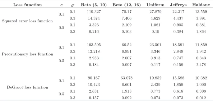
Table 2. Relative eciencies of Bayes estimators relevant to MLE when n = 10, t = 4, and A= 0:1.

Squared error loss function

0.1 0.1 119.327 70.17 27.879 22.217 13.559

0.3 14.374 7.406 4.629 4.437 3.891

0.5 0.1 3.326 2.109 1.081 0.905 0.381

0.3 0.216 0.103 0.19 0.384 1.864

Precautionary loss function

0.1 0.1 103.595 66.52 23.501 18.591 11.859

0.3 12.218 6.991 3.346 2.849 1.942

0.5 0.1 2.953 2.007 0.913 0.747 0.343

0.3 0.184 0.097 0.117 0.159 2.478

DeGroot loss function

0.1 0.1 90.167 63.078 19.852 15.588 10.382

0.3 10.423 6.601 2.439 1.859 1.000

0.5 0.1 2.631 1.913 0.773 0.618 0.308

0.3 0.157 0.092 0.074 0.073 0.012

Table 3. Relative eciencies of Bayes estimators relevant to MLE when n = 10, t = 4, A= 0:8.

Loss function c g Beta (5, 10) Beta (12, 16) Uniform Jereys Haldane Squared error loss function

0.1 0.1 25.634 38.665 212.931 673.934 631.542

0.3 0.187 0.293 0.504 0.539 0.673

0.5 0.1 0.221 0.316 0.832 1.314 3.367

0.3 1.530 2.371 1.623 1.240 0.602

0.1 0.1 28.092 40.798 467.035 6438.339 239.711

0.3 0.204 0.309 0.925 1.438 13.616

0.5 0.1 0.239 0.332 1.278 2.709 1.700

0.3 1.651 2.487 2.165 1.780 0.889

0.1 0.1 31.084 43.163 2004.194 4065.666 121.000

0.3 0.225 0.327 2.610 24.936 1.000

0.5 0.1 0.261 0.350 2.315 9.747 1.000

0.3 1.796 2.615 3.257 3.301 9.000

under SRSWOR, are dened as follows: MSE(^A(ML)) = E(^A(ML) A)2;

MSE(^A(ML))

=Xn

t=0

(^A(ML) A)2_{t!(n t)!}n! t(1 )n t: (17)

MSE(^A(Bayes)Beta)

=

n

X

t=0

(^A(Bayes)Beta A)2_{t!(n t)!}n! t(1 )n t:

(18) MSE(^A(Bayes)Uniform)

=Xn

t=0

(^A(Bayes)Uniform A)2_{t!(n t)!}n! t(1 )n t:

(19) MSE(^A(Bayes)Jereys)

=

n

X

t=0

(^A(Bayes)Jereys A)2_{t!(n t)!}n! t(1 )n t:

(20) MSE(^A(Bayes)Haldane)

=

n

X

t=0

(^A(Bayes)Haldane A)2_{t!(n t)!}n! t(1 )n t:

(21) MSE(^A(Bayes)Mixture)

(9)

=

n

X

t=0

(^A(Bayes)Mixture A)2_{t!(n t)!}n! t(1 )n t:

(22) In order to compare the Bayes estimator with the classical estimator, the Relative Eciency (RE) of Bayes estimators relevant to the classical estimator has been calculated as follows:

RE(Â(Bayes); Â(ML)) =_MSE(^MSE(Â(ML))

A(Bayes)): (23)

The REs of Bayes estimators for two informative Beta prior distributions are calculated through the values of a = 5; b = 10, and a = 12; b = 16 and by three non-informative prior distributions (such as Uniform, Jereys, and Haldane) with respect to the classical estimator by using Eq. (23) for all the selected loss functions. The main purpose of including the non-informative priors is to compare their performances with the informative priors as well as the MLE. The results of REs are given in Tables 2-4. The eciency of each Bayes estimator relevant to MLE is checked by using dierent values of design constants g and c.

From Tables 1-4, several interesting observations can be made:

i. It is noted that the Bayes estimator performs better than the MLE for small-to moderate-sized samples with all possible values of c and g (cf. Tables 2-4);

ii. The informative Beta prior performs better than the non-informative priors do, when the value of A= 0:1 for small to moderate values of c and g

under all the loss functions (cf. Table 1);

iii. The performance of non-informative priors (such as Uniform, Jereys, and Haldane) is quite better

than that of the Beta prior when A > 0:7 for

small- to moderate-sized samples (cf. Table 3); iv. It is observed that the Jereys prior is more

ecient than the other selected priors when the value of n is small and Ais large for all values of

c and g under all the selected loss functions (cf. Table 3);

v. As the values of n and A increase, the

per-formance of Uniform prior under all the loss functions becomes relatively better than that of other priors (cf. Table 4);

vi. It can be seen that all the selected priors perform more eciently under the squared error loss function when the values of n and A are small

for all values of c and g (cf. Tables 2 and 4); vii. When the value of n is moderate and the value

of A is large, then the Uniform and Jeryes

priors perform better under the precautionary and DeGroot loss functions than other priors do (cf. Table 3);

viii. Eciency of the Bayes estimator is slightly af-fected by the sample size and the choice of priors; however, it is aected by the values of c and g (cf. Tables 2-4).

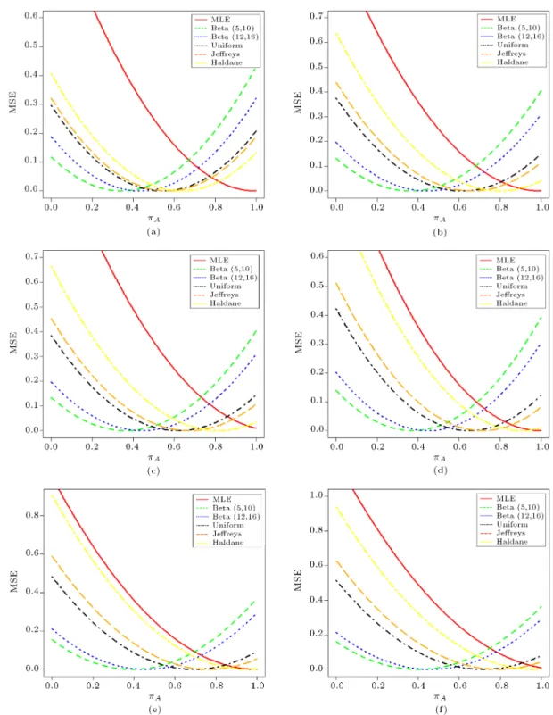
To provide an insight into the proposal, we have also constructed the graph for the comparison of Bayes estimator with the classical estimator for various com-binations c, g, n, and t over the whole range of A(i.e.,

0 A 1). The solid line in these graphs indicates

the behavior of MSE of the MLE, and other lines show the behavior of the Bayes estimators (with dierent priors under dierent loss functions). It is observed from the analysis of Figure 1(a)-(f) that the Bayesian

Table 4. Relative eciencies of Bayes estimators relevant to MLE when n = 50, t = 20, and A= 0:1.

Squared error loss function

0.1 0.1 55.325 49.383 14.130 12.290 10.383

0.3 12.602 7.045 3.451 2.933 1.884

0.5 0.1 1.903 1.679 0.974 0.918 0.309

0.3 0.327 0.147 0.651 1.552 1.000

0.1 0.1 51.509 47.585 13.846 12.144 10.383

0.3 10.863 6.669 2.738 2.218 1.369

0.5 0.1 1.813 1.629 0.920 0.863 0.309

0.3 0.283 0.139 0.418 0.684 1.003

0.1 0.1 47.981 45.858 13.568 12.001 10.383

0.3 9.392 6.314 2.181 1.687 1.000

0.5 0.1 1.727 1.580 0.870 0.811 0.309

(10)

Figure 1. MSE behavior of Bayes estimator and MLE under (a) SELF when c = 0:1; g = 0:3; n = 25; t = 10, (b) PLF when c = 0:1; g = 0:3; n = 25; t = 10, (c) DLF when c = 0:1, g = 0:3, n = 25, t = 10, (d) SELF when c = 0:1, g = 0:3, n = 100, t = 40, (e) PLF when c = 0:1; g = 0:3; n = 100; t = 40, and (f) DLF when c = 0:1, g = 0:3, n = 100, t = 40.

estimators perform better than MLE over the whole range of parameter A. It is found that the Bayes

estimators with Beta priors perform better than the MLE when the value of A 0:4 under all the loss

functions (cf. Figure 1(a)-(c)). The Bayes estimator with non-informative priors (such as Uniform, Jereys, and Haldane) shows better performance than MLE

and the Bayes estimators with informative prior do, when 0:4 < A 0:8 under all loss functions. We

have also presented the MSEs comparison between the Bayes estimators and MLE for a large-sized sample, i.e., n = 100 (cf. Figure 1(d)-(f)). We observed that there is an increase in the performance of MSEs of the Bayes estimators for all the selected priors since

(11)

the value of n is large (cf. Figure 1(a)-(c) versus Figure 1(d)-(f)); however, even then, Bayes estimators outperform the MLE over a range of A starting from

0 to 0.8 for the selected choice of c, g, n, and t. 4.2. Bayes estimators of mixture prior versus

MLE

In order to compare the performances of Bayes estima-tors, we have selected four dierent mixtures of prior distributions. Hussain et al. [29] also used these four sets of prior. The four cases of prior distributions are given as follows:

Case I:

(a1; a2; a3; a4) = (1; 2; 3; 4)

(b1; b2; b3; b4) = (2; 4; 6; 8);

(w1; w2; w3; w4) = (0:3; 0:3; 0:2; 0:2):

Case II:

(a1; a2; a3; a4) = (2; 3; 4; 5)

(b1; b2; b3; b4) = (4; 6; 8; 10);

(w1; w2; w3; w4) = (0:2; 0:3; 0:4; 0:1):

Case III:

(a1; a2; a3; a4) = (3; 4; 5; 6;

(b1; b2; b3; b4) = (6; 8; 10; 12);

(w1; w2; w3; w4) = (0:3; 0:2; 0:1; 0:4):

Case IV:

(a1; a2; a3; a4) = (4; 5; 6; 7);

(b1; b2; b3; b4) = (8; 10; 12; 14);

(w1; w2; w3; w4) = (0:1; 0:3; 0:3; 0:3):

By using Eqs. (17) and (22), we have constructed the graph of the MSEs of the MLE and Bayes estimators for all of the above-mentioned dierent sets of prior distributions. It can be seen that Bayes estimator utilizing the mixture prior performs better than the usual MLE over a wide range of parameter A (cf.,

Figure 2(a)-(d)). It is found that the relative eciency of Bayes estimators is decreased as we make changes in the values of c and g (cf. Figure 2(a) and (b)). We have also noted that as n increases, the eciency of the Bayes estimators decreases; however, still, the Bayes estimator outperforms the MLE in terms of the MSE

(cf. Figure 2(c) and (d)). It is noted that if c = 0:4, g = 0:3, n = 25 and 100, then we have results similar to those of Hussain et al. [29], in which they performed the Bayesian estimation of a Warner [1] model using the mixed prior. Hence, we strongly recommend using a mixed prior in the case of disagreement between researchers about the shape of the distribution of the parameter of the interest.

Therefore, in general, we may conclude that the Bayes estimators perform more eciently than the usual MLE in the case of informative, non-informative, and mixed priors.

5. An application with real data set

In order to give a detailed description of the suggested Bayesian method from a practical point of view, we consider the data collected by Liu and Chow [40] in which they estimated the incidence of induced abortion in Taiwan. Liu and Chow [40] carried out Warner [1] procedure with probability of sensitive question being equal to 0.7 for n = 150 married women in order to determine the proportion of women, who had experi-enced induced abortion. The number of yes responses in the sample is recorded as 60, yielding the sample proportion of yes responses (^) as 0.4. Liu and Chow [40] obtained the maximum likelihood estimate as 0.25. Later on, Winkler and Franklin [17] and Bar-Lev et al. [30] analyzed the same data through the Bayesian analysis using complete and conjugate prior distribu-tions, respectively. The Barabesi and Marcheselli [24] also used the same data for the Bayesian estimation of the two-stage randomized response procedure.

The posterior mean and standard deviation using all the selected prior distributions (such as Beta, Uniform, Jereys, and Haldane) under all loss functions (such as squared error, precautionary and DeGroot) are given in Table 5.

It is noted that the Haldane prior performs more eciently than the other priors under the squared error and precautionary loss functions (cf. Table 5). Based on Table 5, we have observed that the performance of Beta prior is relatively good under the DeGroot loss function. Therefore, we recommend using the Haldane and Beta priors under the squared error, precautionary and DeGroot loss functions, respectively, by using Liu and Chow [40] data for practical consideration. 6. Summary and conclusions

In this study, a Bayesian estimation of a general class of a randomized response model was developed based on simple and mixture priors under dierent loss functions. The comparison between the Bayes estimators and MLE was made based on MSE. The analysis reveals that the performance of the Bayesian

(12)

Figure 2. MSE behavior of Bayes estimator and MLE when (a) c = 0:2, g = 0:4, n = 25, t = 10, (b) c = 0:4, g = 0:3, n = 25, t = 10, (c) c = 0:2, g = 0:4, n = 100, t = 40, and (d) c = 0:4, g = 0:3, n = 100, t = 40.

Table 5. Analysis of Liu and Chow [40] data by assuming c = 0:4, g = 0:3, n = 150, and t = 60.

Priors

Square error loss function

Mean SD Mean SD Mean SD

Beta (5,10) 0.280263 0.074778 0.290068 0.140032 0.300215 0.257796 Beta (12,16) 0.348379 0.065655 0.354512 0.110749 0.360752 0.185199 Uniform 0.254464 0.097577 0.272532 0.190091 0.291882 0.358041 Jereys 0.234750 0.104300 0.256877 0.210369 0.281091 0.406031 Haldane 0.000000 0.000010 0.000006 0.003465 0.328994 1.000000

estimators was quite good for all possible choices of design parameters c and g over the wide range of population proportion A. It was observed that the

superiority of the Bayes estimators was obvious as the sample size decreased. The Bayes estimators with informative prior (such as Beta) and non-informative priors (such as Uniform, Jereys, Haldane) performed

more eciently than MLE when A 0:4 and 0:4 <

A 0:8, respectively, for all values of c and g under

all loss functions. Moreover, the Bayes estimators also showed better performance in the case of mixed prior for small- and moderate-sized samples. Hence, it may be concluded that whenever prior information about the likely values of the parameter of interest is

(13)

available, we should opt for Bayesian approach in order to nd precise and better estimates.

Acknowledgement

The author, Muhammad Riaz, is indebted to King Fahd University of Petroleum and Minerals (KFUPM), Dhahran, Saudi Arabia for providing excellent research facilities. The authors thank the anonymous reviewers and editor for the constructive comments that helped improve the last version of the paper.

References

1. Warner, S.L. \Randomized response: A survey tech-nique for eliminating evasive answer bias", Journal of the American Statistical Association, 60, pp. 63-69 (1965).

2. Greenberg, B., Abul-Ela, A., Simmons, W., and Horvitz, D. \The unrelated question randomized re-sponse: theoretical framework", Journal of the Amer-ican Statistical Association, 64, pp. 529-539 (1969).

3. Moors, J.J.A. \Optimizing of the unrelated question randomized response model", Journal of the American Statistical Association, 66, pp. 627-629 (1971).

4. Kim, M.J., Tebbs, J.M., and An, S.W. \Extension of Mangat's randomized response model", Journal of Statistical Planning and Inference, 36(4), pp. 1554-1567 (2006).

5. Christodes, T.C. \A generalized randomized response technique", Metrika, 57, pp. 195-200 (2003).

6. Hussain, Z. and Shabbir, J. \Improved estimation procedures for the mean of sensitive variable using randomized response model", Pakistan Journal of Statistics, 25(2), pp. 205-220 (2009).

7. Kim, J.-M. and Heo, T.-Y. \Randomized response group testing model", Journal of Statistical Theory and Practice, 7(1), pp. 33-48 (2013).

8. Lee, G.S., Hong, K-H., Kim, J-M., and Son, C-K. \An estimation of a sensitive attribute based on a two stage stratied randomized response model with stratied unequal probability sampling", Brazilian Journal of Probability and Statistics, 28(3), pp. 381-408 (2014).

9. Abdelfatah, S. and Mazloum, R. \Improved random-ized response model using three decks of cards", Model Assisted Statistical Application, 9, pp. 63-72 (2014).

10. Tanveer, T.A. and Singh, H.P. \Some improved ad-ditive randomized response models utilizing higher order moments ratios of scrambling variable", Models Assisted Statistics and Applications, 10(4), pp. 361-383 (2015).

11. Blair, G., Imai, K., and Zhou, Y-Y. \Design and anal-ysis of the randomized response technique", Journal of the American Statistical Association, 110(511), pp. 1304-1319 (2015).

12. Singh, H.P. and Gorey, S.M. \An ecient new random-ized response model", Communications in Statistics-Theory and Methods, 46(24), pp. 12059-12074 (2017).

13. Chaudhuri, A. and Mukerjee, R., Randomized Re-sponse: Theory and Methods, Marcel- Decker, New York (1998).

14. Tracy, D. and Mangat, N. \Some development in randomized response sampling during the last decade-a follow up of review by Chdecade-audhuri decade-and Mukerjee", Journal of Applied Statistical Science, 4, pp. 533-544 (1996).

15. Chaudhuri, A., Randomized Response and Indirect Questioning Techniques in Surveys, Chapman & Hall, CRC Press, Taylor & Francis, Boca Raton, USA (2011).

16. Chaudhuri, A. and Christodes, T.C. Indirect Ques-tioning in Sample Surveys, Springer Verlag, Berlin Heidelberg (2013).

17. Winkler, R. and Franklin, L. \Warner's randomized response model: A Bayesian approach", Journal of the American Statistical Association, 74, pp. 207-214 (1979).

18. Migon, H. and Tachibana, V. \Bayesian approxima-tions in randomized response models", Computational Statistics and Data Analysis, 24, pp. 401-409 (1997).

19. Pitz, G. \Bayesian analysis of randomized response models", Journal of Psychological Bulletin, 87, pp. 209-212 (1980).

20. O'Hagan, A. \Bayes linear estimators for randomized response models", Journal of the American Statistical Association, 82, pp. 580-585 (1987).

21. Spurrier, J. and Padgett, W. \The application of Bayesian techniques in randomized response", Socio-logical Methods, 11, pp. 533-544 (1980).

22. Oh, M. \Bayesian analysis of randomized response models: a Gibbs sampling approach", Journal of the Korean Statistical Society, 23, pp. 463-482 (1994).

23. Unnikrishnan, N. and Kunte, S. \Bayesian analysis for randomized response models", Sankhya, 61, pp. 422-432 (1999).

24. Barabesi, L. and Marcheselli, M. \A practical im-plementation and Bayesian estimation in Franklin's randomized response procedure", Communications is Statistics-Simulations and Computation, 35, pp. 365-373 (2006).

25. Barabesi, L. and Marcheselli, M. \Bayesian estimation of proportion and sensitivity level in randomized re-sponse procedures", Metrika, 72, pp. 75-88 (2010).

26. Hussain, Z. and Shabbir, J. \Bayesian estimation of population proportion of a sensitive characteristic us-ing simple Beta prior", Pakistan Journal of Statistics, 25(1), pp. 27-35 (2009).

(14)

27. Hussain, Z. and Shabbir, J. \Bayesian estimation of population proportion in Kim and Warde (2005) mixed randomized response using mixed prior distribution", Journal of Probability and Statistical Science, 7(1), pp. 71-80 (2009).

28. Hussain, Z. and Shabbir, J. \Estimation of the mean of a socially undesirable characteristics", Scientia Iran-ica, 20(3), pp. 839-845 (2013).

29. Hussain, Z., Shabbir, J., and Riaz, M. \Bayesian estimation using Warner's randomized response model through simple and mixture prior distributions", Com-munications in Statistics-Simulations and Computa-tions, 40(1), pp. 147-164 (2011).

30. Bar-Lev, E.S., Bobovich, K., and Boukai, B. \A com-mon conjugate prior structure for several randomized response models", Test, 12(1), pp. 101-113 (2003).

31. Adepetun, A.O. and Adewara, A.A. \Bayesian analysis of Kim and Warde randomized response technique using alternative priors", American Journal of Com-putational and Applied Mathematics, 4(4), pp. 130-140 (2014).

32. Hussain, Z., Abid, M., Shabbir, J., and Abbas, N. \On Bayesian analysis of a general class of randomized response models in social surveys about stigmatized traits", Journal of Data Science, 12(4), pp. 1-21 (2014).

33. Son, C.-K. and Kim, J.-M. \Bayes linear estimators of two stage and stratied randomized response models", Models Assisted Statistics and Applications, 10, pp. 321-333 (2015).

34. Song, J.J. and Kim, J-M. \Bayesian estimation of rare sensitive attribute", Communications in Statistics-Simulation and Computation, 46(5), pp. 4154-4160 (2017).

35. Legendre, A., New Methods for the Determination of Orbits of Comets, Courcier, Paris (1805).

36. Gauss, C.F., Least Squares Method for the Combi-nations of Observations, (translated by J. Bertrand 1955), Mallet-Bachelier, Paris (1810).

37. Norstrom, J.G. \The use of precautionary loss func-tions in risk analysis", IEEE Transaction Reliability, 45, pp. 400-403 (1996).

38. DeGroot, M.H., Optimal Statistical Decision, McGraw-Hill Inc, New York (1970).

39. Chaubey, Y. and Li, W. \Comparison between max-imum likelihood and Bayes methods of estimation for binomial probability with sample compositing", Journal of Ocial Statistics, 11, pp. 379-390 (1995).

40. Liu, P.T. and Chow, L.P. \The eciency of the multi-ple trial randomized response model", Biometrics, 32, pp. 607-618 (1976).

Biographies

Muhammad Abid obtained his MSc and MPhil degrees in Statistics from Quaid-i-Azam University, Islamabad, Pakistan in 2008 and 2010, respectively. He did his PhD in Statistics from the Institute of Statistics, Zhejiang University, Hangzhou, China in 2017. He served as a Statistical Ocer in National Accounts Wing, Pakistan Bureau of Statistics (PBS) during 2010-2011. He is now serving as an Assistant Professor at the Department of Statistics, Government College University, Faisalabad, Pakistan from 2017 to present. He has published more than 15 research papers in research journals. His research interests include statistical quality control, Bayesian statistics, non-parametric techniques, and survey sampling. Aisha Naeem obtained MSc degree in Statistics from University of Agriculture, Faisalabad, Pakistan in 2003 and MPhil degree in Statistics from Government College University, Faisalabad, Pakistan in 2014. She is serving as an Assistant Professor at the Department of Statistics, Government Degree College, Samanabad, Faisalabad, Pakistan. Her research interests include randomized response models and Bayesian statistics. Zawar Hussain received his PhD degree in Statis-tics from the Quaid-i-Azam University, Islamabad, Pakistan. Currently, he is an Associate Professor of Statistics in Quaid-i-Azam University, Islamabad, Pakistan. He has published 90 research papers in re-search journals. His rere-search interests include sampling techniques, randomized response models, and Bayesian statistics.

Muhammad Riaz obtained his PhD in Statistics from the Institute for Business and Industrial Statis-tics, University of Amsterdam, The Netherland in 2008. He is a Professor at the Department of Mathematics and Statistics, King Fahd University of Petroleum and Minerals, Dhahran, Saudi Arabia. His current research interests include statistical process control, non-parametric techniques, and experimental design. Muhammad Tahir obtained his PhD in Statistics from Quaid-i-Azam University, Islamabad, Pakistan, in 2017. Currently, he is an Assistant Professor of Statis-tics in Government College University, Faisalabad, Pakistan. He has published more than 25 research papers in national and international reputable journals. His research interests include Bayesian reputed infer-ence, reliability analysis, and mixture distributions.