Element Free Galerkin Mesh-Less Method for
Fully Coupled Analysis of a Consolidation Process
M.N. Oliaei
1and A. Pak
1;Abstract. A formulation of the Element Free Galerkin (EFG), one of the mesh-less methods, is developed for solving coupled problems and its validity for application to soil-water problems is examined through numerical analysis. The numerical approach is constructed to solve two governing partial dierential equations of equilibrium and the continuity of pore water, simultaneously. Spatial variables in a weak form, the displacement increment and excess pore water pressure increment, are discretized using the same EFG shape functions. An incremental constrained Galerkin weak form is used to create the discrete system equations and a fully implicit scheme is used to create the discretization of the time domain. Implementation of essential boundary conditions is based on penalty method. Examples are studied and the obtained results are compared with closed-form or nite element method solutions to demonstrate the capability of the developed model. The results indicate that the EFG method is capable of handling coupled problems in saturated porous media and can predict well, both soil deformation and the variation of pore water pressure, over time.
Keywords: Mesh-less; EFG; Penalty method; Soil-water coupled problem; Consolidation process.
INTRODUCTION
The Finite Element Method (FEM) is well estab-lished for modelling complex problems in engineering science. It is a developed technique, but it is not without shortcomings. The reliance of the method on a mesh leads to complications for certain classes of problem. Diculties are encountered when mesh distortion deals with FEM. Considerable loss in accu-racy arises in problems of large deformations, crack propagation, phase transformation, movement of free surface, strain localization and shell problems. The use of a mesh in modelling these problems creates diculties in the treatment of discontinuities, which do not coincide with original mesh lines. This is due to the essential properties of an element-based shape function.
One solution for such a problem is to remesh the problem domain and use an adaptive algorithm in com-putation. This remeshing process is time-consuming
1. Department of Civil Engineering, Sharif University of Tech-nology, P.O. Box 11155-9313, Tehran, Iran.
*. Corresponding author. E-mail: [email protected]
Received 24 September 2006; received in revised form 4 March 2007; accepted 30 April 2007
and sometimes causes mesh-size dependent results (for example, the crack tip problem of creep). Projection of eld variables between meshes in successive stages of the problem, leads to logistical problems, as well as a degradation of accuracy. In addition, for large, three-dimensional problems, the computational cost of remeshing at each step of the problem becomes prohibitively expensive.
One eective numerical method is meshless method that does not require any element for shape function construction. Meshless methods have ap-peared as connectivity free between elements and nodes.
There are a number of mesh-less or mesh-free methods that have been proposed and have achieved remarkable progress in recent years. For example, Smooth Particle Hydrodynamics (SPH) [1,2]; the Fi-nite Dierence Method with arbitrary irregular grids (FDM) [3,4]; the Diuse Element Method (DEM) [5]; the Element Free Galerkin (EFG) method [6], which is a developed version of DEM; the Reproducing Kernel Particle Method (RKPM) [7], which is an improved version of SPH; hp-clouds [8,9]; Partition of Unity FEM (PUFEM) [10]; the Finite Point Method (FPM) [11]; boundary node methods [12]; the Mesh-less Local
Petrov-Galerkin (MLPG) method [13]; the Point In-terpolation Method (PIM) [14]; the Point Assembly Method (PAM) [15]; boundary point interpolation methods [16]; the Least Squares Collocation Mesh-Less (LSCM) method [17] and so forth.
Among these methods, the EFG method has been applied to various types of boundary value prob-lem, which contain the above-mentioned numerical diculties. The shape functions that are obtained by the Moving Least Square (MLS) approximation, based on nodes (not elements), are both consistent and compatible. They are of a higher order than those used in ordinary FEM, because they are polynomials. These higher order shape functions eectively induce more accurate approximations.
This paper presents a formulation for the element free Galerkin method to solve two-dimensional coupled problems in saturated soil. The authors' goal is to emphasize the benets of this formulation in solving of coupled problems in the eld of geotechnical engi-neering.
The rst attempt to apply such mesh-less strate-gies to a soil-water coupled problem was made by Modaressi et al., using a coupled EFG(DEM)-FEM technique with Lagrange multipliers [18]. In their work, the displacement of a porous-solid skeleton is modelled by a standard FEM, while uid pure pressures are included as element{free nodes. Another mesh-less strategy by Wang et al. [19,20]), based on PIM or radial PIM, has also been applied to solve Biot's consolidation problem for elastic material under innitesimal strain, in order to overcome the disadvantage of the lack of delta function properties in the shape functions obtained by MLS approximation in the EFG method. Nogami et al. [21] incorporated the double porosity model into the radial PIM to analyze lumpy clay lling. The arrangement of the current paper is as follows. Following the introduction, in EFG shape function construction, MLS approximation and weight function implementation is stated along with a ow chart. In the third section, the weak form is developed through a global equilibrium in soil-water system at each time-step. Then, spatial variables, displacement increments and excess porewater pressure increments are discretized by the same EFG shape functions. A fully implicit scheme in the time domain is used to avoid spurious ripple eects. At the end of this section, an algorithm for numerical solution is pro-posed for solving coupled problems, based on EFG. The fourth section presents the numerical analysis of two coupled problem in geotechnical engineering and compares the results with closed-form and numerical (FEM) solutions, in order to examine the accuracy of the description of the present algorithm. The problems are 1D and 2D consolidation, respectively. Conclusion follows in the last section.
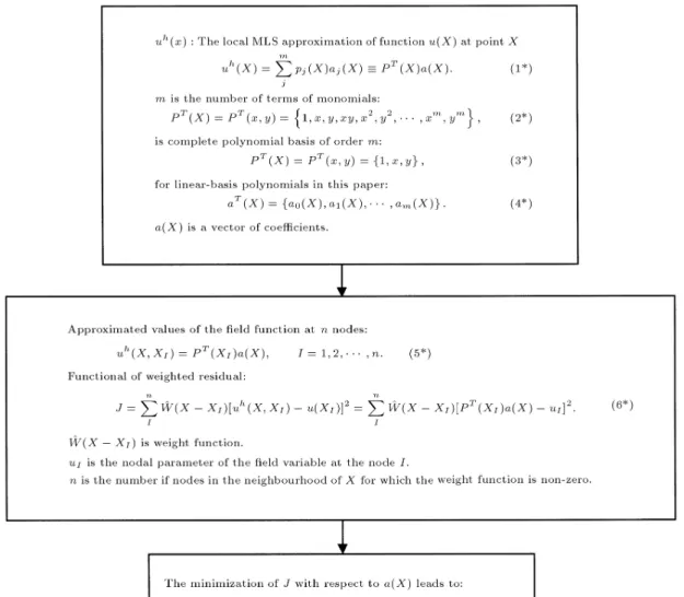
EFG SHAPE FUNCTION CONSTRUCTION The EFG method is used to establish a system of equations for the whole problem domain, without the use of a predened mesh. EFG uses a set of nodes scattered within the problem domain, as well as a set of nodes scattered on the boundaries of the domain to represent (not discretize) the problem domain and its boundaries. So, construction of the shape functions is only based on the nodes.
The EFG method employs MLS approximants to approximate the function. These approximants are constructed from three components: A weight function of compact support associated with each node; a basis usually consisting of a polynomial; and a set of coecients that depend on position. The weight function is nonzero only over a small subdomain around a node, which is called its support. The support of the weight function denes a node's inuence domain, which is the subdomain over which a particular node contributes to the approximation. The overlap of the nodal inuence domains denes the nodal connectivity. One attractive property of MLS approximants is that their continuity is related to the continuity of the weight function; therefore, a low order polynomial ba-sis, e.g., a linear baba-sis, may be used to generate highly nonlinear continuous approximations by choosing an appropriate weight function. Thus, post processing to generate smooth elds of eld variables derivatives, which is required for C0 FEM, is unnecessary in EFG.
Since the shape function can be constructed with arbitrary continuity, the boundaries of the node sup-ports do not aect deleteriously the smoothness of the shape function.
The arbitrary overlaps of the nodal supports lead to a variable connectivity: The number of nodes aecting the approximation varies from point to point arbitrarily, and is usually higher than that for the FEM. In the Moving Least Squares (MLS) approxima-tion, the weight function takes its maximum value over each desired point in the domain wherein the unknown function should be evaluated, but in the Weighted Least Squares (WLS) approximation, the peak of the weight function is placed only on distributed nodes.
In the WLS method, the set of coecients is constant in each subdomain and the approximation order is, directly, the order included in the set of basis functions. On the other hand, in the MLS approach, the set of coecients are a function of position and the resultant unknown function may include higher order functions.
There is another important characteristic of the MLS approach. The shape functions of this method are global and can be used all over the domain.
Although MLS approximation is both consistent and compatible, the use of MLS approximation
pro-duces shape functions that do not possess the Kro-necker delta function property, which implies that one cannot impose essential boundary conditions in the same way as in conventional FEM.
To conquer this problem, in this paper, the penalty method [22] is used to create a constrained Galerkin weak form for the imposition of essential boundary conditions. The use of the penalty method produces equation systems of the same dimensions that conventional FEM produces for the same number of nodes; the modied stiness matrix is still positive denite, banded and symmetric and the treatment of boundary conditions is as simple as it is in conventional FEM.
MLS Approximation
Moving Least Squares (MLS), originated by mathe-maticians for data tting and surface construction, is often termed local regression and loss [23]. Nayroles et al. [5] were the rst to use the MLS procedure to construct shape functions for DEM. DEM was modied by Belytschko et al. [6], as the EFG method, where the MLS approximation is also employed. The invention of DEM and the advances in EFG have had a great impact on the development of mesh-less methods. The MLS approximation has two major futures that make it popular:
1. the approximated eld function is continuous and smooth in the entire problem domain;
2. it is capable of producing an approximation with the desired order of consistency.
In this paper, the procedure of constructing shape functions for EFG, using MLS approximation, based on the work of Belytschko et al. [6], is stated in Figure 1.
An important ingredient in the EFG method is the weight function. The weight function should be non-zero only over a small neighbourhood of XI, called
the inuence domain of node I, in order to generate a set of sparse discrete equations. This is equivalent to stating that the weight functions have compact support. The precise character of the weight function seems to be unimportant, although it is almost manda-tory that it be positive and increase monotonically as the distance between the evaluation point and the node decreases. Furthermore, it is desirable that the weight function be smooth: If the weight function is C1continuous, then, for a polynomial basis, the shape
function is also C1 continuous.
The choice of weight function aects the result-ing approximation, uh(X). Constant weight function
over the entire domain and constant weight function with compact support cannot result in ecient MLS approximation, but continuous weight function with
compact support, where they are smooth functions that cover larger subdomains such that (n > m), results in ecient MLS approximation that is used in the EFG method; the approximation is continuous and smooth, even though the polynomial basis is only linear, since the approximation inherits the continuity of the weight function.
Note that most mesh-less weight functions are bell-shaped. Among these weight functions, the cubic spline weight function has been tested and worked very well for many applications. As it has basically been adopted for various kinds of computation, this weight function has been used in the authors' EFG code. FORMULATION
In this section, rst, the weak form is developed and then discretization of the weak form is stated. At the end of this section, an algorithm for numerical implementation of the EFG code is proposed.
Weak Form
Two sets of governing equations for soil-water coupled problems are given as follows [24,25]:
Equilibrium equation:
ij;j+ bi= 0; (1)
where ij is total stress tensor; and biis body force
vector.
Continuity equation of uid ow:
r:(v) G = @(n)@t ; (2)
where:
density of uid;
v velocity vector of uid ow; G uid mass ux from sink or source; n porosity of soil mass; and
t time.
In this formulation, the uid is pore water, so the density of the uid is considered constant. Assuming that the sink or source term may be con-sidered later as a boundary condition, the continuity equation of the pore water is written in the following form.
Continuity equation of pore water ow: r:(v) = @n
@t: (3)
This is the same as the incompressibility equation of the solid-water mixture in the Biot consolidation theory [26].
Terzaghi's eective stress principle:
ij= ij0 pij; (4)
where 0
ij is eective stress tensor (tension positive);
is Biot coecient ( 1); p is excess pore water pressure increment (compression positive); and ij
is kronecker delta.
Note that, for consistency between two govern-ing equations, p is considered to be positive when compressive.
Constitutive law for soil skeleton:
0
ij= Dijkl("kl+13csklp); (5)
where Dijkl is material matrix; "kl is total strain
increment tensor; and cs is compressibility of solid
particles of soil.
Darcy's law for ow in porous media: vi= Kij
y +p
;j; (6)
where Kij is permeability tensor of soil skeleton; y
is elevation head; p is pore water pressure; and is unit weight of water.
Boundary conditions:
{ For the soil skeleton boundary: (
ui= ui on u[0; 1)
ijnj = ti on t[0; 1)
(7) { For the uid boundary:
(
p = p on
p[0; 1)
vi= vi on v[0; 1) (8)
where:
ui displacement vector;
ui the boundary value of displacement; u displacement boundary;
nj the unit normal vector at the boundary;
ti the boundary value of traction; t traction boundary;
p excess pore pressure;
p the boundary value of pore pressure;
p pore pressure boundary;
vi velocity vector;
vi the boundary value of velocity; and v velocity (ux) boundary.
Initial conditions: (
ui= uijt=0 on 0
p = pjt=0 on 0 (9)
where is the domain.
By applying the Weighted Residual Method (W.R.M) on Equation 1 and inserting Equations 4, 5 and 7 -Appendix A- the soil skeleton should satisfy the following constrained Galerkin weak form of the equilibrium equation:
Z
(Lu)
TD
ijkl"kld
Z
(u)
Tb
id
Z
t
(u)Tt
td
Z
(Lu)
T
ijpd
+ Z
(Lu)
T(1=3)c
sDijklklpd
Z
u
(1=2)(u u)T
pu(u u)d
= 0; (10)
where:
(u) test function; L dierential operator; u incremental displacements;
u prescribed incremental displacements on the essential boundary; and
pu penalty factor for equilibrium equation weak
form.
Note that, in the weak form, incremental displace-ments, (u), relate to the incremental displacements in an x; y direction. So, u must be considered as a vector.
u =
u v
: (11)
According to the time domain discretization methods, the following relation can be used for eld function f in the time interval [t; t + t]:
f = (1 )ft+ ft+t= ft+ f: (12)
can vary from zero (fully explicit scheme) to 1.0 (fully implicit scheme). The approximation is uncondition-ally stable when 0:5, but for any value of 6= 1, the numerical solution can exhibit a spurious ripple eect [20].
Time integration is applied to Equation 3 and, by using the weighted residual method and inserting Equations 6 and 8 - Appendix A - the weak form for state variables in the continuity equation of the pore water is expressed as:
Z
v
(p)T(v
ini)d +
Z
(Lpp)
TK i2d
+ Z
(LpP )
T(K
ij=)pi;jd
+ Z
(LpP )
T(K
ij=)p;jd
+ Z (P ) T(@n=@t)d + Z p
(1=2)(p p)T
pp(p p)d = 0;
(13) where:
(p) test function; Lp dierential operator;
p excess pore water pressure increment; p prescribed excess pore water pressure increment on the essential boundary; pp penalty factor for the continuity
equation weak form. Numerical Discretization
Displacement increments (u; v) and excess pore water pressure increment (p), at any time and at any point, are approximated using Equation 7* (Figure 1), so:
uh=u
v h
=Xn
I
'I 0
0 'I
uI
vI
=Xn
I
IuI; (14)
and:
ph=Xn I
'IpI: (15)
Dierential operator matrices L and Lp are given by:
L = 2
4@=@x0 @=@y0 @=@y @=@x 3
5 ; (16)
and: Lp=
@=@x @=@y
: (17)
By using Equations 14 to 17, the products of Luh
and Lpph become:
Luh=Xn I
2
4'I;x0 '0I;y 'I;y 'I;x
3 5uI
vI
=Xn
I
BIuI;
(18)
and: Lpph=
n X I 'I;x 'I;y pI =
n
X
I
BpIpI: (19)
Note that pu is a diagonal matrix of penalty factors
which is as follows: pu=
pu1 0
0 pu2
: (20)
The penalty factors can be a function of coordinates and can be dierent from each other. However, in practice, they are often assigned identical constants of a large positive number for each set of equations. ppis
also a scalar penalty factor. The imposition of essential boundary conditions is described in Appendix B.
Substituting Equations 14, 15, 18 and 20 into Equation 10, after a lengthy manipulation, the fol-lowing system of equations can be obtained for the equilibrium equation:
[KG11+ Ku]U + KG12P = FGu+ Fu: (21)
Again, by substituting Equations 15 and 19 into Equation 13, and with consideration of:
"v= n
X
I
'I;x 'I;y uvI I
=Xn
I
CIuI; (22)
after a lengthy manipulation, the following system of equations can be obtained for the continuity equation: KG21U + [KG22+ Kp]P = FGp+ Fp: (23)
Equations 21 and 23 are the nal system of discrete equations for the entire problem domain. These equations should be solved simultaneously for a fully coupled model. As shown, both equations contain the same state variables that are displacement increments and the excess pore water pressure increment. The matrix equation in coupled form can be written as:
KG11+ Ku KG12
KG21 KG22+ Kp
U P
=
FGu+ Fu
FGp+ Fp
: (24)
The non-diagonal terms in the matrix, [K], of Equa-tion 24 represent the coupling terms in the analysis. KG12 represents the force induced by pore pressure
and KG21 represents the uid ow caused by ground
deformation.
In Equation 24, KG11, KG12, KG21, KG22 are the
parts of the global stiness matrix assembled using the nodal stiness matrices. Their dimension are (2nt; 2nt), (2nt; nt), (nt; 2nt), (nt; nt), respectively;
where nt is the total number of nodes in the entire
problem domain. K
u, Kp are the global penalty
ma-trices assembled using the nodal penalty mama-trices. U and P are the global displacement increments vector and the global excess pore pressure increment vector, respectively. Their dimensions are 2nt, nt, respectively.
FGu, FGp are the global force increments vector
and the global uid ux increment vector, respectively.
F
u, Fp are the global penalty vectors. The global
vectors collect the relative nodal vectors at all nodes in the entire problem domain.
The nodal matrices and vectors that form system of discrete equations are all summarized below:
K11ij =
Z
B
T
i DBjd; (25)
K12ij =
Z
B
T
i (1=3)csDm'jd
Z
B
T
i m'jd;
(26) where `m' represents ij in vector form, i.e.:
m =1 1 0T; (27)
K21ij =
Z
'iCjd; (28)
K22ij = t
Z
B
T
pi(Kw=)Bpjd; (29)
where `Kw' represents the permeability tensor, i.e.:
Kw=
Kx 0
0 Ky
; (30)
Fui =
Z
T
i bd +
Z
t
T
i td ; (31)
Fpi = t
Z
B
T
piKw2d
t Z
B
T
pi(Kw=)Bpipid
t Z
v
'ivTinid ; (32)
where: Kw2=
0 Ky
; (33)
and pi is pore pressure of node i.
In Fpi, the rst and second terms are the
ows due to changes in velocity, while the third term
indicates the eect of a specied ux on the boundaries. K
uij =
Z
u
T
ipujd ; (34)
K pij =
Z
p
'ipp'jd ; (35)
F
ui =
Z
u
T
i puud ; (36)
F
pi =
Z
p
'ipppd : (37)
Numerical Implementation
The sequence of the numerical algorithm for the 2D-EFG code is, briey, as follows:
1. Dene the geometrical dimensions and properties (material, plane strain or plane stress condition, permeability, etc) of the domain;
2. Set up the nodal points;
3. Determine the inuence domain of each node; 4. Set up quadrature cells in the domain and
quadra-ture lines on the essential and natural boundaries (displacement and pore pressure - traction and uid ux);
5. Set up all Gauss points, weights and Jacobian for each cell and line over the background mesh; 6. Set up the initial displacement, the initial pore
pressure at the nodal points and the stress levels at the Gauss points;
7. Loop over the time steps;
8. Loop over the Gauss points to assemble the K matrix and F vector in Equation 24.
(a) Select the neighboring nodes for a Gauss point based on the inuence domain of the nodes; (b) Determine the shape functions and shape
func-tion derivatives for the nodes; (c) Evaluate the nodal matrices/vectors;
(d) Assemble the nodal contribution to the global matrices/vectors;
(e) End loop.
9. Solve the system equation to obtain the displace-ment incredisplace-ments and excess pore water pressure increment at each node;
10. Recalculate the displacement increments and excess pore water pressure increments at each node, using the MLS shape function based on nodes in a local domain to achieve more accuracy;
11. Determine nodal displacements and pore water pressure;
12. Evaluate strain, stress and uid velocity at each cell Gauss point;
13. Evaluate eective stress on nodal points by inter-polation;
14. Record the history of state variables and their derivatives;
15. Back to 7; 16. End.
NUMERICAL ANALYSIS
The examples in this section are selected for bench-marking the code demonstrating the capability to solve fully coupled hydro-mechanical problems.
One-Dimensional Consolidation
For validation process, the developed code is exam-ined rst for solving the 1D Terzaghi's consolidation problem. A saturated layer of soil, with a thickness H = 10 m and large horizontal extent, rests on a rigid, impervious base. This is a 1D problem, so, a certain width is sucient for modeling (Figure 2). The EFG model is a regular nodal arrangement (21 nodes in height and 11 nodes in a 2.5 m width). In the model, only the upper surface is permeable and the rest is impervious. The bottom is xed for dis-placement, while two sides are xed against horizontal displacements only. The soil matrix is homogeneous and behaves elastically with E = 10000 Kpa and v = 0. A constant surcharge, = 20 Kpa, is suddenly applied to the surface of the soil layer and the initial state of the problem is set to a uniform pore pressure P0= 20 Kpa.
Figure 2. One-dimensional consolidation problem.
With time, the uid drains through the surface layer, transferring the load from the uid to the soil matrix. The closed form solution of 1D Terzaghi's consolidation problem is as follows [27]:
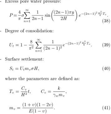
- Excess pore water pressure: P =4
1
X
n=1
1 2n 1sin
(2n 1)y 2H
e (2n 1)2 2 4 Tv:
(38) - Degree of consolidation:
Ut= 1 82 1
X
n=1
1
(2n 1)2e (2n 1)
2 2
4 Tv: (39)
- Surface settlement:
St= UtmvH; (40)
where the parameters are dened as: Tv=HCv2t; Cv= k
wmv;
mv= (1 + )(1 2)E(1 ) : (41)
The following criterion is used to maintain stability and freedom from oscillation [19,28]:
h2
6Cv t
h2
2Cv; (42)
where h is the characteristic size of the node distance. For the 1D model, h is the nodal spacing.
A constant permeability of Ky = 510 8 m/s is
used, while the value of Kx is considered zero.
Analytical and numerical results are plotted in Figures 3 through 6. The variation of surface settle-ment is plotted in Figure 3 and the history of excess
Figure 3. Surface settlement history for 1D consolidation problem.
pore water pressure is plotted in Figure 4 for 5 sample points. They are all in excellent agreement with closed form solutions. It is also shown in Figure 4 that the essential boundary condition for the pore pressure on the surface of soil layer (y=H = 0) is imposed exactly by the penalty method. In Figure 5 isochrone curves give
Figure 4. Pore water pressure dissipation history for 1D consolidation problem.
Figure 5. Normalized isochrones for 1D consolidation problem.
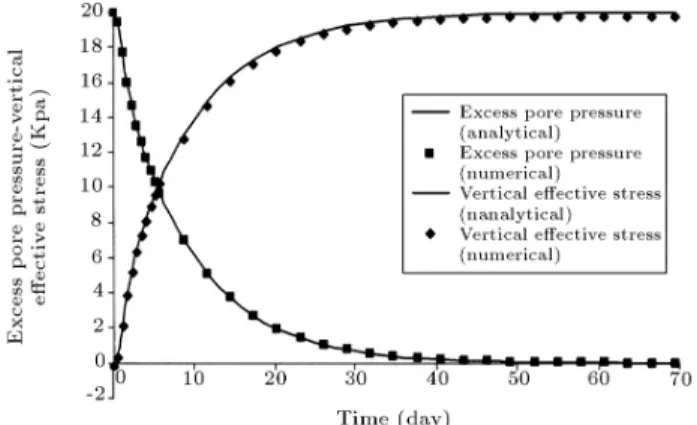
Figure 6. Histories of pore water pressure and eective stress at mid-height of soil layer for 1D consolidation problem.
the spatial distribution of excess pore water pressure at dierent times. The transfer of pore pressure to eective stress is illustrated in Figure 6. It is seen that the eective stresses are less accurate than pore pressures. The reason is that the eective stresses are obtained from vertical total stresses at each node, using the derivatives of the displacement eld as the state variable, while the pore pressure is the state variable itself.
Two-Dimensional Consolidation
Most consolidation problems of practical interest are two or three dimensional, so the one dimensional solu-tions provided by the Terzaghi consolidation theory are useful only as indicators of settlement magnitudes and rates. This problem here examines a two dimensional plane strain consolidation case: The settlement and pore pressure histories of a partially loaded strip of soil, which is assumed to be linear elastic. This particular case is chosen because an exact solution is available for this 2D consolidation problem [29]. Furthermore, for comparison of the accuracy of EFG results with FEM results, the last ones are obtained by ABAQUS as well.
A schematic model of a partially loaded strip of soil is shown in Figure 7.
The material properties assumed for this analysis are as follows: Young's modulus is chosen 690 Gpa (108 lb/in2); the Poisson ratio is 0; the material's
permeability in both horizontal and vertical directions is 5:0810 7m/day (2:010 5in/day); and the specic
weight of the pore uid was chosen as 272.9 KN/m3
(1.0 lb/in3).
The applied load has a magnitude of 3.45 Mpa (500 lb/in2). The strip of soil is assumed to lie on
a smooth, impervious base. The top surface is fully drained and the rest of the boundaries are all imper-vious. For displacement boundaries, the horizontal base boundary xes the vertical freedom and vertical boundaries x the horizontal freedom. Note that the left vertical boundary is a symmetry line. A regular arrangement of nodes (4111) is used for the EFG
model.
Validation of the settlement of the surface on the symmetry line is plotted in Figure 8, where it is
compared with the exact solution of Gibson et al. [29] and the FEM results of ABAQUS. There is very good agreement between the EFG results and the theoretical and nite element solutions. Also, it is seen that the EFG results are more accurate than the FEM solutions. As mentioned earlier, the reason relates to the concept of weight function in the EFG.
The dissipation history of excess pore pressure on the symmetry line at the mid-height of the soil layer is shown in Figure 9. The EFG and FEM results are in good agreement. As shown, at initial consolidation times, an increase in the pore pressure will be induced in the sample. Subsequently, the pore pressure falls. This eect was pointed out by Mandel [30] as an eect in 2D. It was also predicted by Cryer [31], thus, it is known as the Mandel-Cryer eect and was demonstrated experimentally by Verruijt [32].
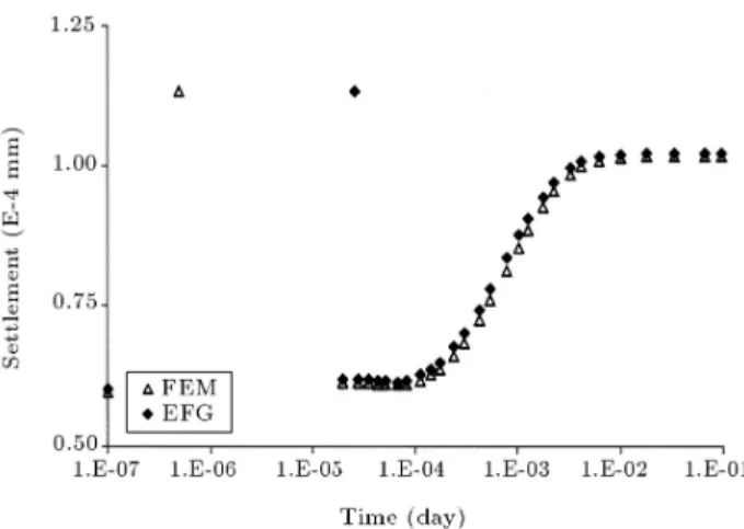
For midpoint on the symmetry line, when time of about 0.01 days elapses, the dissipation of excess pore water pressure is almost complete and settlement reaches its stable state, as shown in Figure 10.
Figure 8. Surface settlement history on the symmetry line for 2D consolidation problem.
Figure 9. History of pore uid pressure at mid-height of soil layer on the symmetry line for 2D consolidation problem.
Figure 10. Settlement history at mid-height of soil layer on the symmetry line for 2D consolidation problem.
In this problem, the computation speed for EFG is 1.11 times slower compared to the FEM's.
Since the EFG with the penalty method does not increase the size of the system equation and the stiness matrix is banded, the computational eort is approximately the same order as that of FEM for this problem, in which the number of nodes is 451.
The computational eort of EFG may increase for a large number of eld nodes. The reasons are: (1) Much time is used for computing the EFG shape functions compared with the FEM shape functions; (2) The number of integration points is needed in EFG compared with FEM to guarantee an accurate solution.
It worths noting that the principle attraction of the EFG method is the possibility of simplify-ing adaptivity and simulatsimplify-ing problems with movsimplify-ing boundaries and discontinuities, which compensates the computational eort of the EFG method, with respect to that of FEM.
CONCLUSIONS
The details of the Element Free Galerkin (EFG) mesh-less method and its numerical implementation have been presented in this paper to study the numerical solution of the coupled problem of consolidation in geotechnical engineering. The numerical results show the accuracy of the method to be better than that achievable with the nite element method.
The results of the examples indicate EFG validity, and capability for analyzing coupled problems in sat-urated porous media. From this study, the following conclusions can be drawn.
First, EFG is an eective method to discretize spatial variables (displacement and excess pore water pressure). Unlike other mesh-less methods, EFG has a simple shape function and construction of the spatial derivatives, due to the polynomial basis and weight
function, are easy. Essential boundary conditions can be easily implemented, using the penalty method.
Second, using the same order of shape functions for displacement and excess pore water pressure is ecient to avoid spatial oscillation, if a fully implicit scheme in the time domain is used.
Third, since the weakform developed in this paper is an incremental Galerkin weak form, so it can be used improved for nonlinear problems.
REFERENCES
1. Lucy, L. \A numerical approach to testing the ssion hypothesis", Astron. J., 82, pp. 1013-1024 (1977). 2. Gingold, R.A. and Monaghan, J.J. \Smooth
parti-cle hydrodynamics: theory and applications to non-spherical stars", Mon. Not. R. Astron. Soc., 181, pp. 375-389 (1977).
3. Liszka, T. and Orkisz, J. \The nite dierence method at arbitrary irregular grids and its application in applied mechanics", Computer. Struct., 11, pp. 83-95 (1980).
4. Jensen, P.S. \Finite dierence techniques for variable grids", Comput. Struct., 2, pp. 17-29 (1980).
5. Nayroles, B., Touzot, G. and Villon, P. \Generalizing the nite element method: Diuse approximation and diuse elements", Comput. Mech., 10, pp. 307-318, 1992.
6. Belytschko, T., Lu, Y. Y. and Gu, L. \Element free Galerkin methods", Int. J. Numer. Meth. Eng., 37, pp. 229-256 (1994).
7. Liu, W.K., Adee, J. and Jun, S. \Reproducing kernel and wavelet particle methods for elastic and plastic problems", in Advanced Computational Methods for Material Modeling, D.J. Benson, Ed., 180/PVP 268 ASME, pp. 175-190 (1993).
8. Oden, J.T. and Abani, P. \A parallel adaptive strategy for hp nite element computations", TICAM Rep. 94-06, University of Texas, Austin (1994).
9. Armando, D.C. and Oden, J.C. \Hp clouds- A meshless method to solve boundary value problems", TICAM Rep. 95-05, University of Texas, Austin (1995).
10. Babuska, I. and Melenk, J.M. \The partition of unity nite element method", Technical Report Technical Note BN-1185, Institute for Physical Science and Technology, University of Maryland (April 1995). 11. Onate, E. et al. \A nite point method in
com-putational mechanics and applications to convective transport and uid ow", Int. J. Numer. Meth. Eng., 39, pp. 3839-3866 (1996).
12. Mukherjee, Y.X. and Mukherjee, S. \Boundary node method for potential problems", Int. J. Numer. Meth. Eng., 40, pp. 797-815 (1997).
13. Atluri, S.N. and Zu, T. \A new meshless local Petrov-Galerkin (MLGP) approach in computational mechan-ics", Comput. Mech., 22, pp. 117-127 (1998).
14. Liu, G.R. and Gu, Y.T. \A point interpolation method", in Proc. 4th Asia-Pacic Conference on Computational Mechanics, December, Singapore, pp. 1009-1014 (1999).
15. Liu, G.R. \A point assembly method for stress analysis for solid", in Impact Response of Materials and Struc-tures, V.P.W. Shim et al., Eds., Oxford University Press, Oxford, pp. 475-480 (1999).
16. Liu, G.R. and Gu, Y.T. \Coupling of element free Galerkin method with boundary point interpolation method", in Advances in Computational Engineer-ing and Science, S.N. Atluri and F.W. Brust, Eds., ICES'2K, Los Angeles, pp. 1427-1432 (Aug. 2000). 17. Zhang, X., Liu, X.H., Song, K.Z. and Lu, M.W. \Least
squares collocation meshless method", Int. J. Numer. Meth. Eng., 51, pp. 1089-1100 (2001).
18. Modaressi, H. and Aubert, P. \Element-free Galerkin method for deforming multiphase porous media", Int. J. Numer. Meth. Eng., 42, pp. 313-340 (1998). 19. Wang, J.G., Liu, G.R. and Lin, P. \A point
inter-polation method for simulating dissipation process of consolidation", Comput. Meth. Appl. Mech. Eng., 190, pp. 5907-5922 (2001).
20. Wang, J.G., Liu, G.R. and Lin, P. \Numerical analysis of Biot's consolidation process by radial point interpo-lation method", Int. J. Solids & Structures, 39, pp. 1557-1573 (2002).
21. Nogami, T., Wang, W. and Wang, J.G. \Numerical method for consolidation analysis of lumpy clay llings with meshless method", Soils and Foundations, 44(1), pp. 125-142 (2004).
22. Liu, G.R. and Yang, K.Y. \A penalty method for enforce essential boundary conditions in element free Galerkin method", in Proc. 3rd HPC Asia'98, Singa-pore, pp. 715-721 (1998).
23. Lancaster, P. and Salkauskas, K. \Surfaces generated by moving least squares methods", Math. Comput., 37, pp. 141-158 (1981).
24. Bathe, K.J., Finite Element Procedures in Engineering Analysis, Prentice-Hall, Inc., Englewood Clis, N.J., Chapter 4, pp. 114-194 (1982).
25. Thomas, G.W., Principles of Hydrocarbon Reservoir Simulation, Tabir publishers (1977).
26. Biot, M.A. \General theory of three-dimensional con-solidation", J. Appl. Phys., 12, p. 155 (1941). 27. Terzaghi, K. and Peck, R.B., Soil Mechanics in
Engi-neering Practice, 2nd Ed., John Wiley &, Sons, New York (1976).
28. Vermeer, P.A. and Verruijt, A. \An accuracy condition for consolidation by nite elements", Int. J. Numer. Analy. Meth. Geo., 5, pp. 1-14 (1981).
29. Gibson, R.E., Schiman, R.L. and Pu, S.L. \Plane strain and axially symmetric consolidation of a clay layer on a smooth impervious base", Quarterly Journal of Mechanics and Applied Mathematics, 23, pt. 4, pp. 505-520 (1970).
30. Mandel, J. \Consolidation des sols (etude mathema-tique)", Geotechnique, 3, pp. 287-299 (1953).
31. Cryer, C.W. \A comparison of three-dimensional con-solidation theories of biot and terzaghi", Quart. J. Mech. and Appl. Math., XVI(4), pp. 401-412 (1963). 32. Verruijt, A. \Discussion", Proc. 6th Int. Conf. Soil
Mechanics and Foundation Engineering, 3, Montreal, pp. 401-402 (1965).
APPENDIX A
Derivation of Weak Forms
Weighted residual method is employed to obtain the weak forms:
The weak form of the equilibrium equation (Equa-tion 1):
Z
(ij;j+ bi)!d = 0; (A1)
where ! is the test function (it is a variation of the displacement increment - (u)- for the equilibrium equation).
Integration by parts of Equation A1 leads to the following equation:
Z
ijnj!d
Z
ij!;jd+
Z
bi!d=0:(A2)
Now, by substituting boundary conditions (Equa-tion 7) in Equa(Equa-tion A2, one obtains:
Z
t
ti!d +
Z
u
(1=2)(u u)T
pu(u u)d
Z
ij!;jd +
Z
bi!d = 0:(A3)
By applying Terzaghi's eective stress principle (Equation 4) in Equation A3, the following is ob-tained:
Z
t
ti!d +
Z
u
(1=2)(u u)T
pu(u u)d
Z
0
ij!;jd +
Z
pij!;jd
+ Z
bi!d = 0: (A4)
Inserting the constitutive law for the soil skeleton (Equation 5) into Equation A4 the following is
obtained: Z
t
ti!d +
Z
u
(1=2)(u u)T
pu(u u)d
Z
Dijkl"kl!;jd
Z
Dijkl(1=3)csklp!;jd
+ Z
pij!;jd +
Z
bi!d = 0:(A5)
By employing the Galerkin method:
! = (u); !;j = (Lu): (A6)
Substituting Equation A6 into A5 and, after rear-rangement, the constrained Galerkin weak form of the equilibrium equation (Equation 10) is obtained. The weak form of the continuity equation of the pore
water ow (Equaiton 3) is as follows: Z
(vi;i+ _n)!
0d = 0; (A7)
where !0 is test function. (It is a variation of the
pore pressure increment - (p)- for the continuity equation.)
Integration by parts yields: Z
vini!0d
Z
vi! 0 ;id +
Z
_n!
0d = 0: (A8)
Substituting boundary conditions (Equation 8) in Equation A8 yields the following:
Z
v
vini!0d +
Z
p
(1=2)(p p)T
pp(p p)d
Z
vi! 0 ;id +
Z
_n!
0d = 0: (A9)
Considering Darcy's law for ow in porous media (Equation 6) and inserting Equation 12 leads to:
vi= Kij
y +p
;j = Ki2 (Kij=)p;j
= Ki2 (Kij=)(pt+ p);j: (A10)
By employing the Galerkin scheme:
!0 = (p); !
;i= (Lpp); (A11)
and substituting Equations A10 and A11 into Equa-tion A9 and, after rearrangement, the constrained Galerkin weak form of the continuity equation of pore water (Equation 13) is obtained.
APPENDIX B
Imposition of Essential Boundary Conditions Due to the lack of Kronecker delta function properties in the MLS shape function, there is a dierence between the displacement of MLS approximation and the prescribed displacement on the essential boundary. The same concept exists for prescribed pore pressure on the essential boundary:
u 6= u; on u; p 6= p; on p: (B1)
Therefore, the test functions of (u) and (p) are not equal to zero on the essential boundaries for the weak forms of the equilibrium equation and continuity equations, respectively, which are in contrast to the conventional FEM. In FEM, for the Kronecker delta function properties, the test functions, (u) and (p), are equal to zero on the essential boundaries. Hence, in FEM, the curve integrals on in the weak forms (Equations A2 and A8 in Appendix A) will change to the curve integrals on t and v
(Equa-tions A3 and A9), and the curve integrals on u and p will be zero in these equations.
To penalize the dierence between the approximated and the prescribed state variables on essential boundaries in EFG, the terms,
R u(1=2)(u u)T
pu(u u)d and
R p(1=2)(p p)T
pp(p p)d , are added to
the weak forms (Equations 10 and 13) to introduce the constrained Galerkin weak form using the penalty method. These terms are produced by the penalty method for handling essential boundary conditions for cases when u u 6= 0 and p p 6= 0. They can be viewed physically as smart terms that can force u u = 0 and p p = 0. If the trial functions, u and p, can be so chosen that u u = 0 and p p = 0 (similar to FEM), the smart terms will be zero and the added terms will vanish completely.
Considering the term R u(1=2)(u u)T
pu(u u)d , the following can be written:
Z
u
(1=2)(u u)T
pu(u u)d
= Z
u
(u)T
pu(u u)d
= Z u (u)T puud Z u (u)T
puud : (B2)
Substituting the expression of the MLS approximation
for the displacement increment of Equation 14 into Equation B2 the following is obtained:
Z u n X I
IuI
!T pu
n
X
J
JuJ
! d Z u n X I
IuI
!T puud = n X I n X J
(uI)T
Z
u
T
IpuJd
uJ n
X
I
(uI)T
Z
u
T
Ipuud
= n X I n X J
(uI)T(KuIJ)uJ
n
X
I
(uI)T(FuI)
= nt X I nt X J
(uI)T(KuIJ)uJ
nt
X
I
(uI)T(FuI); (B3)
where K
uIJ and FuI are nodal penalty matrix and
nodal penalty vector for the weak form of the equilib-rium equation, respectively; and ntis the total number
of nodes in the entire problem domain. (Note that, in the weak form, the integration is over the entire problem domain, and all the nodes can be involved. Therefore, the summation limits have to be changed to nt).
Finally we have:
nt X I nt X J
(uI)T(KuIJ)uJ
nt
X
I
(uI)T(FuI)
= (U)T(K
uU Fu): (B4)
In which K
u and Fu are the global penalty matrix
and the global penalty vector for the weak form of the equilibrium equation, respectively; which are imple-mented in the system Equation 21 for the equilibrium equation.
A similar approach is used for implementation of K
p and Fp in the system Equation 23 for the