An Ecient Procedure for Computing an Optimal
(R,Q) Policy in Continuous Review Systems with
Poisson Demands and Constant Lead Time
N. Yazdan Shenas
1, A. Eshraghniaye Jahromi
1;and M. Modarres Yazdi
Abstract. In this paper, a continuous review inventory system is considered in which an order in a batch of size Q is placed immediately after the inventory position reaches R. Transportation time is constant and demands are assumed to be generated by a stationary Poisson process with one unit demand at a time. Demands not covered immediately from the inventory are backordered. In a recent paper, the exact evaluation of batch-ordering policies for two-level inventory systems was derived. This evaluation is based on a recursive procedure for determining the exact policy costs in case of one-for-one replenishment policies. In this paper, we show how this result can be applied to nd the optimal solution of a (R; Q) policy. To obtain the optimal policy for this system, considering a one-for-one policy, we will rst solve the base stock model by setting the inventory position at the supplier to a certain value. By considering ordering cost, we next derive the cost function of the dened (R; Q) model and nd the optimal solution for the exact value of the expected system costs using a search method. In demonstrating the applicability of the proposed method, we resort to solving an example.
Keywords: Inventory; Continuous review; (R; Q) model; Base stock model; Poisson demand; Optimal solution; Backordered demand; Constant lead time.
INTRODUCTION
Stochastic inventory model have received considerable attention in inventory literature. We consider one of the most common practical stochastic inventory control problems, known as the continuous (R; Q) model. In this system, a batch of size Q is ordered when the inventory position declines to R. The model and some of its variants have been analyzed by several authors [1,2].
The basic assumptions of the classical (R; Q) can be found in Hadley and Whitin [3]. The optimal solution of this problem and other related problems can be determined by various techniques [4,5]. In practice, however, it is most common to use a simple two-step approximation. In the rst step, the batch quantity Q is determined in a deterministic model.
1. Department of Industrial Engineering, Sharif University of Technology, Tehran, P.O. Box 11155-9414, Iran.
*. Corresponding author. E-mail: [email protected]
Received 18 November 2007; received in revised form 16 April 2008; accepted 14 June 2008
One such approach is to determine the order quantity according to the standard EOQ model. Axsater [6] and Gallego [7] have derived bounds for approximation errors when using such techniques.
In a (R; Q) inventory system with backordering, there are several approximations to the average inven-tory level. Lau and Lau [8] presented a comparison of dierent methods for estimating the average inventory level in this type of system.
Axsater [9] considered a (R; Q) policy with con-stant lead time. The demand during lead-time demand is assumed to be normally distributed. There are standard ordering and holding costs as well as a so-called ll rate constraint. The problem is to determine the reorder point R and the order quantity Q so that the total expected costs are minimized. He suggested another equally two-step approach and both R and Q were assumed to be continuous variables.
Axsater [10] also considered a warehouse facing a compound Poisson customer demand. Normally, the warehouse replenishes from an outside supplier, according to a continuous review reorder point policy.
However, it is also possible to use emergency orders. Such orders incur additional costs, but have a much shorter lead time. He considered standard holding and backorder costs as well as ordering costs. A heuristic decision rule for triggering emergency orders was suggested.
Modularization and customization have made en-terprises face multi-item inventory problems and the interaction between those items. A powerful and aordable information technology system can make the continuous review inventory policy more convenient, ecient and eective. Others have introduced dier-ent aspects of cost into their models such as design problems or exibility in the assembly sequence. The aforementioned considerations make models more com-plex and the closed form solutions cannot be obtained. Thus, iterative algorithms must be used to nd a near optimal solution. Several studies have presented some ecient solution procedures to obtain the approximat-ing decision rules for such problems [11,12].
Wang and Hu [13] developed a (R; Q) model to nd the optimal lot size and reorder point for a multi-item inventory with interactions between necessary and optional components. In order to accurately approxi-mate costs, the service cost is introduced and dened as a proportion of the service level. In addition, the service and purchasing costs are taken simultaneously and are treated as a budget constraint for executives to consider because the rm's strategy could inuence the choice of service level. They formulated the proposed model as a nonlinear optimization problem, when the service level is nonlinear.
A recent (R; Q) model was presented by Lau and Lau [14]. When an order for an out-of-stock inventory item is received, sometimes a xed cost independent of the order size is incurred to expedite the order. They showed that the current standard \textbook formulation" for this situation contains a number of conceptual aws. An improved formulation is presented, followed by explanations of computation procedures and numerical illustrations.
There are several studies in which the (R; Q) policy is applied in multi-echelon inventory systems. Axsater [15] considered an inventory system with one warehouse and some identical retailers. Lead times are constant and the retailers face independent Poisson demand. When the retailers need to replenish their stocks, they order batches from the supplier and, in the same way, the warehouse replenishes its stock by ordering batches from an outside source. Solving the mentioned inventory system, Axsater extended his previous results in [16], where replenishments are a one-for-one policy. He provided simple recursive procedures for determining the holding and shortage costs of dierent one-for-one policies.
Here, we consider the continuous review
inven-tory system that is controlled using a (R; Q) pol-icy. Demands are assumed to be generated by a stationary Poisson process with one unit demand at a time. Unlled demand is backordered and the cost for a backorder is proportional to the delay until delivery takes place. The transportation time is constant.
As mentioned before, Axsater [15,16] derived the procedures for determining the best solution for a one-for-one and a batch-ordering policy in a two-level inventory system. Setting the inventory position at the supplier to a certain value, we show how these procedures can be used for nding the optimal solution of base stock and (R; Q) policies.
Our approach uses an inventory cost function that reects costs incurred on an average unit. The relative advantage of the approach in this paper is that it focuses directly on evaluating the average costs associated with a stockage policy. Earlier approaches focus on characterizing the steady-state behavior of the inventory levels and then use the steady state distribution (or an approximation thereof) to deter-mine the average costs associated with the stockage policy. Axsater [16] mentions that this approach is more ecient and direct at nding the optimal stock policy for the assumed (traditional) cost function; it appears to be the only available approach when the cost is given by a nonlinear function of either the delays experienced by the customer or the unit's storage time at each of the facilities.
The rest of the paper is organized as follows: In the next section, the one-for-one replenishment policy and its assumptions are described and a problem formulation is presented in detail. Then, we show how the result of the one-for-one replenishment policy in a two-level inventory system can be used for the exact evaluation of the base stock policy. Following that, the batch-ordering policy in a two-level inventory system is extended by considering order costs for both retailer and supplier. Setting the inventory position at the supplier to a certain value, a search algorithm for nding the optimal solution of a (R; Q) policy is presented. Then, for demonstrating the applicability of the proposed method, we resort to solving an example. Finally, some remarks concerning possible extension are made.
DESCRIPTION AND PROBLEM FORMULATION
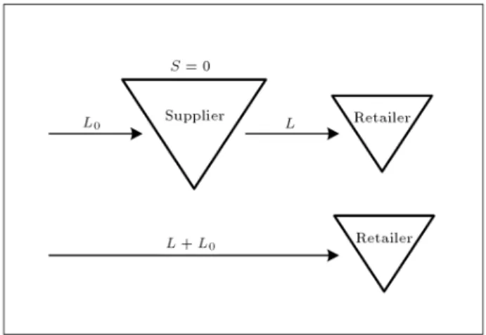
Consider an inventory system that consists of one sup-plier and one retailer, as shown in Figure 1. The retailer faces stationary and independent Poisson demand with one-unit demand at a time. Unlled demand is backordered and the shortage cost is considered just for the retailer. The retailer and the supplier carry
Figure 1. Inventory system.
inventory and replenish their stock according to a one-for-one policy, i.e. when a demand occurs, one unit is immediately ordered from the supplier and the supplier orders one unit at the same time. It means essentially that it is assumed that ordering costs are low and can be disregarded. Delayed demands and delayed orders are satised on a rst come, rst serve basis. The transportation time from the supplier to the retailer and the replenishment lead time from the outside source to the supplier are constant (i.e. the outside source has ample capacity).
A one-for-one replenishment policy is completely characterized by determination of the inventory posi-tions at the retailer and at the supplier.
Considering the one-for-one policy, we will solve the base stock model by setting the inventory position at the supplier to a certain value and then nding the optimal solution for this model.
DERIVING THE COST FUNCTION AND FINDING THE OPTIMAL SOLUTION FOR THE BASE STOCK MODEL
In the base stock model, when a demand occurs at the retailer, one unit is immediately ordered from the outside source. We denote the base stock policy by (RB; 1), i.e. when inventory position declines
to RB one unit is ordered. This base stock policy
is completely characterized by determination of the retailer's reorder point. The ordering cost per time unit in all base stock policies with one unit demand at a time is constant, and thus is not considered in the analysis. In this section, we try to nd the optimal value of RB as a decision variable.
We convert the assumed one-for-one model to the dened base stock model (Figure 2). To nd the optimal value of RB, our approach uses the optimal
retailer inventory position in the inventory system with the one-for-one policy, when setting the value of the inventory position at the supplier to 0.
Lemma 1.
A one-for-one replenishment system with S, S0= 0, L
and L0 is the same as a base stock system with lead
time L + L0 and RB= S 1.
Figure 2. The equivalent systems based on Lemma 1.
Proof
When a demand occurs at the retailer, one unit is immediately ordered from the supplier and the supplier orders one unit at the same time. When demand occurs, the supplier is empty; because the inventory position at the supplier is zero, the supplier receives the ordered unit after L0time units (all the outstanding
orders are assigned before they arrive at the supplier and the supplier must order new one to assign to the new one ordered), and it is received by the retailer L time units away. Therefore, an order placed by the retailer arrives after L0+ L time units.
Based on Lemma 1, if S minimizes the cost
function of the assumed one-for-one replenishment system, R
B = S 1 will minimize the cost function
of the base stock system. It is easy to conclude that we can disregard policies with a negative inventory position for the retailer in the assumed one-for-one ordering system when looking for the optimal solution. Therefore, conne ourselves to the case where S 0 for the base stock model.
To evaluate the total holding and shortage costs per time unit when applying one-for-one ordering policies (i.e. c(S0; S)), we use the method introduced
by Axsater [15,16] (see Appendix).
The total cost of the assumed one-for-one replen-ishment system can be calculated by Equation A13:
c(0; S) = (S(0) + (0)): (1)
Considering Equations A4 and A8, it is easy to simplify Expression 1 as:
c(0; S) = S(L
0): (2)
It means that if S minimizes
S(L0), it will minimize
c(0; S). In order to optimize S(L
0), we need to
determine the S that minimizes S(L 0).
Based on Equations A5 and A6, we can derive: 1(L
0) 0(L0) = e (L+L0)h + ; (3)
S+1(L
0) S(L0) = S(L0) S 1(L0)+
e (L+L0)h +
(L + L0)SS
S! ; S > 0: (4) Using Equation 4, it is easy to conclude that S(L0)
is convex in S. Furthermore, we obtain the following expression:
S+1(L
0) S(L0) =h + S
X
k=0
e (L+L0)
(L + L0)kk
k!
=h + P (S; (L + L0)) ;
S 0: (5)
Based on convexity specications, the optimal value of S that minimizes S(L0) will be the minimum value of
S that is valid for:
P (S; (L + L0)) + h : (6)
Therefore, the optimal value of RB in a base stock
system with lead time L + L0 will be S 1 where S
minimizes the cost function of the assumed one-for-one replenishment system.
DERIVING THE COST FUNCTION AND FINDING THE OPTIMAL SOLUTION FOR THE LOT SIZE-REORDER POINT MODEL In this section, we try to nd the optimal value of the reorder point and lot size as decision variables. In the rst part of this section, the cost function for a lot size-reorder point model is developed and extended by considering the order cost for the retailer. In the second part of this section, for a given lot size, the optimal value of the retailer's reorder point will be found, and nally in the last part of this section, a search method to nd the optimal solution of the lot size-reorder point model will be provided. These three sub sections are presented as follows:
Cost Function for the Lot Size-Reorder Point Model
The cost function for a serial system that consists of a retailer and a supplier is developed in Axsater [15].
In this system, both facilities apply a lot size-reorder point policy, where Rw and Qware in units of Q. The
average cost per time unit, that is valid for Rw 1,
is determined by averaging over the individual units in a warehouse batch:
C =Q1
wQ
RWX+Qw
j=Rw+1
R+QX k=R+1
c(jQ; k); Rw 1: (7)
In developing the model, Axsater [15] made a few assumptions. He assumed that the order lot sizes at the retailer and the supplier are given and xed, therefore the order costs have been eliminated from the cost function (Equation 7). It means that the ratio of order cost to unit holding cost at the supplier and the ratio of order cost to unit holding and shortage costs at the retailer are negligible. In cases where shipping and handling are signicant, this assumption is violated.
We extend the model by considering the order costs of both the retailer and the supplier (Figure 3). By considering the rates of orders, the expected total holding and shortage and order costs per time unit can be written as:
C0=A0
QwQ+
A Q+ 1
QwQ
RWX+Qw
j=Rw+1
R+QX k=R+1
c(jQ; k); Rw 1: (8)
Lemma 2
A serial system that consists of one retailer and one supplier and the retailer applies the (R; Q) policy and the supplier applies (Rw; Qw) where Rwand Qware in
units of Q with Rw = 1; Qw = 1; A0 = 0; L and L0
is the same as a lot size-reorder point system with lead time L + L0where the retailer applies (R; Q).
Proof
When the inventory position at the retailer reaches R, one order (of size Q) is immediately ordered from the supplier and the supplier orders one order (in the same size) at the same time. When demand occurs, the supplier is empty because the inventory position at the supplier is zero, the supplier receives the ordered unit after L0 time units (all the outstanding orders
are assigned before they arrive at the supplier and the supplier must order new ones to assign to the new one ordered), and it is received by the retailer L time units away. Therefore, an order placed by the retailer arrives after L0+ L time units.
So, if Rw; Qw and A0 are replaced with specied
values in Lemma 2, we will have: T C(Q; R) =A
Q +
1 Q
R+QX k=R+1
c(0; k): (9)
Optimal Value of the Retailer's Reorder Point for a Given Lot Size
In order to optimize the lot size-reorder point model for a given lot size, we need to determine the R that minimizes the system costs, according to Equation 9. Note that, for a given Q, we can optimize T C(Q; R) by optimizingPR+Qk=R+1c(0; k) with respect to R. Further-more, it is possible to show that optimal policies for lot size-reorder point models are such that R Q. For k 0, it was proven that c(0; k) is convex in k. Using Equations A5 and A6 in the same way, it is easy to show that c(0; k) is convex at all values of k. Therefore, PR+Q
k=R+1c(0; k) will be convex in R.
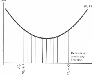
The optimal retailer's reorder point for a given lot size Q is denoted by R
Q. As shown in Figure 4, RQ
is a point wherein there is a set of Q sequential points
Figure 4. R
Qand the optimal set of Q sequential points
are exactly after this point.
exactly after this point, where the sum of the values of c(0; k) for all members of this set is the minimum of the sum of the values of c(0; k) for all members of any set of Q sequential points.
For simplicity, we set R
1 = RB. Based on c(0; k)
convexity, it is obvious that R
1+ 1 2 [RQ+ 1; RQ+ Q],
therefore we have: R
1 Q + 1 RQ R1: (10)
If R 1, by using Equation 5, we get:
R+Q+1X k=R+2
c(0; k)
R+QX k=R+1
c(0; k) =
(h + )
R+QX k=R+1
P (k; (L + L0)) Q: (11)
The optimal value of R that minimizesPR+Qk=R+1c(0; k) will be the minimum value of R that is valid for:
R+QX k=R+1
P (k; (L + L0)) (h + )Q ; R 1: (12)
If R < 1, by using Equations A5 and A6, it can be shown:
R+Q+1X k=R+2
c(0; k)
R+QX k=R+1
c(0; k) =
(h + )
R+QX k=0
P (k; (L + L0)) Q: (13)
The optimal value of R that minimizesPR+Qk=R+1c(0; k) will be the minimum value of R that is valid for:
R+QX k=0
P (k; (L + L0)) (h + )Q ; R < 1: (14)
Therefore, for a given order size Q, the optimal value of R that minimizes T C(Q; R) will be found by examining values of R starting from R
1 Q + 1 to the rst value
of R that is valid for Equation 14 (for the values less than -1), and then Equation 12 (for the values greater than or equal to -1), respectively.
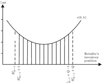
Furthermore, it may also be of interest to utilize R
Q 1 for nding RQ (Figure 5). Note that, when we
have R
Q 1, we found the set of Q 1 sequential points
exactly after this point, where the sum of the values of c(0; k) for the all member of this set, is minimum. When we try to nd R
Q, we try to add one member
(except the selected Q 1 points) to this set, where the values of c(0; k) for the new member is minimum. Based on the convexity of c(0; k), the new member will
Figure 5. Utilizing R
Q 1for nding RQ.
be a point exactly before or after the selected Q 1 sequential points. Considering the R
Q denition, it
can be concluded that: R
Q 2 [RQ 1 1; RQ 1]: (15)
If R
Q= RQ 1, it means that RQ 1+Q is added to (Q
1) members that minimize PRQ 1+Q 1
k=R
Q 1+1 c(0; k) and, if
R
Q = RQ 1 1, it means that RQ 1is the Qth member
of this set. Therefore, we get: c(0; R
Q 1) c(0; RQ 1+ Q) ! RQ= RQ 1 1;
c(0; R
Q 1) > c(0; RQ 1+ Q) ! RQ= RQ 1: (16)
A Search Method to Find the Optimal
Solution of the Lot Size-Reorder Point Model To nd the optimal solution of the lot size-reorder point model, it is necessary to determine R and Q that minimize the system costs, according to Equation 9. This cost function is comprised of two parts. The rst part is a decreasing function on Q which is smaller than or equal to A, and the second part is an increasing function on Q (where R = R
Q), that is larger than or
equal to c(0; R 1+ 1).
Let Qu denote the minimum value of Q that is
valid for: A + c(0; R
1+ 1) Q1u R
QuX+Qu
k=R Qu+1
c(0; k): (17)
Considering the increasing function specications and Expression 17, for Q Qu, we have:
T C(1; R
1) =A + c(0; R1+ 1) Q1 R
Q+Q
X
k=R Q+1
c(0; k)
<AQ +Q1
R Q+Q
X
k=R Q+1
c(0; k) = T C(Q; R): (18) It means that Qu is an upper bound for Q. In the
calculations, it may also be of interest to utilize that: S(L
0) = h + S 1X k=1
P (k; (L + L0))
+
L + L0 S
; S > 0; (19)
which follows directly from Equation A5. Meanwhile from Equations 9 and 16, it is possible to conclude that:
T C(Q + 1; R
Q+1) = (Q T C(Q; RQ)+
min(c(0; R
Q); c(0; RQ + Q + 1)))=Q + 1): (20)
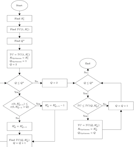
Finally, we can provide a search method, based on the suggested relations, to nd the optimal solution of the lot size-reorder point policies (Figure 6). This method is described by the following owchart shown in Figure 6.
Roptimium and Qoptimium are the optimal values
of the reorder point and lot size in a (R; Q) policy, respectively.
EXAMPLE
In this section, we will try to show the applicability of our search method by solving a test problem. We have assumed that the value of the parameters A; L; L0; h; h0; and are constant and for instance
are as:
A = 10; L = 1; L0= 1; h = 1;
h0= 0:1; = 10 and = 1:
For a base stock model, the optimal value of RB with
lead time L+L0will be S 1, where Sis the minimum
value of S that is valid for Expression 6, i.e.: P (4; 1 (1 + 1)) 10 + 110 ! S= 4 ! R
B = 3:
Based on Equation 9, for computing T C(Q; R), we need to calculate the values of c(0; k). Using Equa-tions 2, 19 and A6, these values can be found easily.
Figure 6. The suggested method to nd the optimal solution of lot size-reo point problems.
As an example, we have:
c(0; 1) = 30; c(0; 0) = 20; c(0; 1) = 11:4887; c(0; 2)=5:9548; c(0; 3)=3:3982; c(0; 4)=2:8266; c(0; 5) = 3:2474:
As said before, R
1 = RB, therefore R1 = 3. Using
Expression 16, we can get R 2:
c(0; R
1) > c(0; R1+ 2) ! R2= R1= 3:
In the same way, we can calculate R
Q for any value of
Q. Using Expression 17, the upper bound for Q can be determined:
T C(1; R
1) = 1 10 + c(0; 4)
= 12:8266 281 X1+28
k= 1+1
c(0; k) = 13:0714 ! Qu= 28; R
Qu = 1:
Finally, from Equation 20, we can compute T C(Q; R Q)
for any value of Q from 1 to Qu.
T C(2; R
2) = 8:0370;
T C(3; R
3) = 6:4907;
T C(4; R
4) = 5:8843; ;
T C(28; R
The minimum value of T C(Q; R
Q) will determine the
optimal policy in the above example, i.e.: Roptimum= 2; Qoptimum= 5;
T C(Qoptimum; Roptimum) = 5:7105:
CONCLUSION
In this paper, we considered a continuous review inventory system that was controlled using a (R; Q) policy. Demands were assumed to be generated by a stationary Poisson process with one unit demand at a time. Unlled demand was backordered and the cost for a backorder was proportional to the delay until delivery took place. The transportation time was constant.
First, we solved the base stock model. To derive the cost function of the system, the one-for-one model in a two-level inventory system was converted to this base stock model. For nding the optimal value of the retailer's reorder point in the base stock model, our approach used the optimal retailer inventory position in the inventory system with the one-for-one policy, when setting the value of the inventory position at the supplier to 0.
Then, the batch-ordering policy in a two-level inventory system was extended by considering two order costs for retailer and supplier. Setting the inventory position at the supplier to a certain value, a search algorithm for nding the optimal solution of a (R; Q) policy was provided.
Earlier approaches focus on characterizing the steady-state behavior of the inventory levels of a stock-age policy and then use the steady state distribution (or an approximation thereof) to determine the average costs associated with the stockage policy. The proposed approach is more ecient and direct at nding the op-timal stockage policy for the traditional cost function. For this reason, the proposed approach can be used when the cost is given by a nonlinear function of either the delays experienced by the customer, or the unit's storage time at the retailer.
NOMENCLATURE
RB retailer's reorder point in an inventory
system with base stock policy, S0 supplier inventory position in an
inventory system with a one-for-one ordering policy,
S retailer inventory position in an inventory system with a one-for-one ordering policy,
L transportation time from the supplier to the retailer,
L0 transportation time from the outside
source to the supplier,
demand intensity at the retailer h holding cost per unit per time unit at
the retailer,
h0 holding cost per unit per time unit at
the supplier,
shortage cost per unit per time unit at the retailer,
R the retailer reorder point, Q the retailer batch size,
Rw the warehouse reorder point (in units
of retailer batches),
Qw the warehouse batch size (in units of
retailer batches),
A xed order cost at the retailer, A0 xed order cost at the supplier,
S(S
0) the expected retailer inventory carrying
and shortage costs, which is incurred to ll a unit of demand at the retailer when applying one-for-one ordering policies with S0 and S as the supplier
and the retailer inventory positions, respectively,
(S0) the average warehouse holding cost
per unit when applying one-for-one ordering policies with S0 as the
supplier inventory positions, S(L
0) the expected retailer inventory
carrying and shortage costs which is incurred to ll a unit of demand at the retailer when applying one-for-one ordering policies with S as the retailer inventory positions and L0as the delay
encountered at the supplier level, c(S0; S) the total holding and shortage costs per
time unit when applying one-for-one ordering policies with S0 and S as
the supplier and the retailer inventory positions, respectively,
T C(Q; R) the total cost per time unit for the retailer when the retailer applies a (R; Q) policy with lead time L + L0,
p(u; ) probability mass function of Poisson with mean ,
P (u; ) cumulative probability distribution function of Poisson with mean . REFERENCES
1. Dura0n, A., Gutie0rrez, G. and Zequeira, R.I. \A
expe-diting", Int. J. of Prod. Economics, 87, pp. 157-169 (2004).
2. Riezebos, J. \Inventory order crossovers", Intr. J. of Prod. Economics, 104, pp. 666-675 (2006).
3. Hadley, G. and Whitin, T.M., Analysis of Inventory Systems, Prentice-Hall, Englewood Clis, NJ (1963). 4. Federgruen, A. and Zheng, Y.S. \An ecient algorithm
for computing an optimal (R,Q) policy in continuous review stochastic inventory systems", Operations Re-search, 40, pp. 808-813 (1992).
5. Rosling, K. \The square-root algorithm for single-item inventory optimization", Working Paper, Vaxjo University (2002).
6. Axsater, S. \Using the deterministic EOQ formula in stochastic inventory control", Management Science, 42, pp. 830-834 (1996).
7. Gallego, G. \New bounds and heuristics for (Q; R) policies", Management Science, 44, pp. 219-233 (1998).
8. Lau, A.H.L. and Lau, H.S. \A comparison of dierent methods for estimating the average inventory level in a (Q; R) system with backorders", Int. J. of Prod. Economics, 79, pp. 303-316 (2002).
9. Axsater, S. \A simple procedure for determining order quantities under a ll rate constraint and normally dis-tributed lead-time demand", Euro. J. of Operational Res., 174, pp. 480-491 (2006).
10. Axsater, S. \A heuristic for triggering emergency orders in an inventory system", Euro. J. of Operational Res., 176, pp. 880-891 (2007).
11. Ghalebsaz-Jeddi, B., Shultes, B.C. and Haji, R. \A multi-product continuous review inventory system with stochastic demand, backorders, and a budget constraint", Euro. J. of Operational Res., 158, pp. 456-469 (2004).
12. Bhattacharya, D.K. \On multi-item inventory", Euro. J. of Operational Res., 162, pp. 786-791 (2005). 13. Wang, T.Y. and Hu, J.M. \An inventory control
system for products with optional components under service level and budget constraints", Euro. J. of Oper-ational Res, doi:10.1016/j.ejor.2007.05.025 (2007). 14. Lau, A.H.L. and Lau, H.S. \An improved (Q; R) formulation when the stockout cost is incurred on a per-stockout basis", Intr. J. of Prod. Economics, doi:10.1016/j.ijpe.2006.04.022 (2007).
15. Axsater, S. \Exact and approximate evaluation of batch-ordering policies for two-level inventory sys-tems", Operations Research, 41(4), pp. 777-785 (1993). 16. Axsater, S. \Simple solution procedures for a class of two-echelon inventory problems", Operations Re-search, 38(1), pp. 64-69 (1990).
APPENDIX
Evaluation of the One-for-One Ordering Policies
This Appendix is a summary of Axsater [15,16]. Con-sider S0and S as the supplier and the retailer inventory
positions, respectively. We dene (as in Axsater's papers for one retailer and where S0 0) the following
notations:
gS0(t) = Density function of the Erlang (; S0)
distri-bution of the time that the warehouse orders a unit to it is demanded by the retailer, for the one-for-one corresponding system with Poisson demand (see Axsater [16] page 65),
GS0(t) = Cumulative distribution function of gS0(t).
thus:
gS0(t) = S0tS0 1
(S0 1)!e
t; (A1)
and: GS0(t) =
1
X
k=S0
(t)k
k! e t: (A2)
The average warehouse holding cost per unit is: (S0) =h0S0(1 GS0+1(L0))
h0L0(1 GS0(L0)); S0> 0; (A3)
and for S0= 0,
(0) = 0: (A4)
Given the value of random delay at the warehouse is equal to t(S0 0 ! 0 t L0), the conditional
expected cost per unit at the retailer is: S(t) = e (L+t)h +
S 1X k=0
(s k)
k! (L + t)kk +
L + t S
; S > 0; (A5)
(0! = 1 by denition) and: S(t) =
L + t S
; S 0: (A6)
The expected retailer inventory carrying and shortage costs, which was incurred to ll a unit of demand at the retailer, is:
S(S 0) =
L0
Z
0
gS0
0 (L0 t)S(t)dt
+ (1 GS0(L
and:
S(0) = S(L
0): (A8)
Furthermore, for S > 0 and for large values of S0 we
have: S(S
0) S(0): (A9)
The procedure starts by determining S0 such that:
GS0(L
0) < "; (A10)
where " is a small positive number.
The recursive computational procedure is: S(S
0 1) =S 1(S0) + (1 GS0(L0))
(S(0) S 1(0)); S
0> 0; (A11)
and for S 0 it is possible to show that: S(S
0) =GS0(L0)L0 GS0+1(L0)S0
+
L S
; S0> 0: (A12)
The sum of the expected total holding and shortage costs per time unit in an inventory system with a one-for-one ordering policy is: