c
Sharif University of Technology, June 2009
Robot Movements in a Cyclic Multiple-Part Type
Three-Machine Flexible Robotic Cell Problem
I.N. Kamal Abadi
1;and S. Gholami
2Abstract. This paper recognizes thirty-six, potentially optimal robot movement policies, to schedule the movements of a robot in a three-machine exible cell. The robotic cell produces multi-type parts, in which the robot is used as a material handling system. In this manufacturing cell, the machines have operational exibility and can be set up for dierent operations; all parts have three operations. Finding the robot movement policy and sequence of parts to minimize the cycle time (i.e., maximize the throughput) is the aim of this work. It was proved that cycle time calculation, in twelve out of thirty-six policies, are unary NP-complete, and a polynomial time algorithm is introduced that can solve the twenty-four left policies. This paper develops the cycle times of all these thirty six robot movements policies, considering waiting times in a exible three-machine robotic cell with multi-type parts, and introduces a parts sequence under a special condition, in which one of the policies minimizes the cycle time (i.e., maximize throughput). This kind of exibility diers from other research into robotic cells, wherein a machine can process dierent operations. Moreover, we consider cells with multiple part types, which is more realistic than other developed models. Finally, a new mathematical model, based on Petri-nets, was provided for one of the robot movement policies. Furthermore, this mathematical model is also developed for the multi-type part problem.
Keywords: Production scheduling; Cyclic blocking open shop; Flexible robotic cell.
INTRODUCTION
In modern technology, the level of automation in manufacturing industries has increased dramatically. Some examples of these automation progresses are in cellular manufacturing and robotic cells. A growing body of evidence suggests that, in a wide variety of industrial settings, material handling within a cell can be accomplished very eciently by employing industrial robots (see [1]). Among the interrelated issues to be considered in using robotic cells are their designs, the scheduling of robot movements and the sequencing of parts to be produced. If, in a robotic cell, CNC machines are used, it is possible to set up dierent operations on machines. This important property of
1. Department of Industrial Engineering, University of Kurdis-tan, Sanandaj, Iran.
2. Department of Industrial Engineering, Tarbiat Modares Uni-versity, Tehran, P.O. Box 14115-143, Iran.
*. Corresponding author. E-mail: nakhai [email protected] Received 19 May 2007; received in revised form 16 October 2007; accepted 17 February 2008
CNC machines is considered, and the 1-unit cycles of robot movement policies are dened. In most previous studies, ow-shop robotic cells are considered [2]. In this paper, a robotic cell with operational exibility that produces multiple-type parts, is considered and, also, the results of the successful studies of Hall et al. [3,4] and Sriskandarajah et al. [5]. Hall [3] analyzed the complexity of a scheduling problem and showed that two policies out of six possible policies are NP-Complete. In this study, these results are used to show the NP-Completeness of the scheduling problems of twelve out of thirty six possible policies. For calculating the cycle time and waiting times for a given sequence of jobs under these two NP-Complete policies, algorithms are introduced [4]. We introduce a mathematical model, based on Petri-nets, to nd the best sequence of jobs and calculate the cycle time and waiting times for policies, wherein their scheduling problems are NP-Complete. Some instance problems are solved by this mathematical model and the results are il-lustrated. Sriskandarajah et al. [5] have introduced a classication scheme for the complexity of robotic
cell scheduling problems. Finally, according to this classication scheme, some algorithms are proposed to solve this problem. This paper is organized as follows.
In the next section, the literature of the robotic cell scheduling problem is briey reviewed. In the third section, the initial notions and required notations are introduced. Following that, the problem and calcula-tion of cycle times for possible policies are described. In the fth section, the problem is analyzed by Petri-nets and a mathematical model and its calculation results are shown. Finally, the proposed algorithms for solving the problem are described.
LITERATURE REVIEW
The robotic cell problem, wherein a robot is used as a material handling system, has received considerable attention, such as in [6,7] and some other works which were pursued. Sethi et al. [6] suggested the following conjecture.
Sethi's Conjecture
In buerless single-gripper robotic cells producing a single part-type and having identical robot travel times between adjacent machines and identical load/unload times, a 1-unit cycle provides the minimum per unit cycle time in the class of all solutions, cyclic or otherwise.
Sethi et al. [6] proved this conjecture for two-machine robotic cell problems. It is proved that a 1-unit cycle solution is optimal over the class of all solutions, cyclic or otherwise. For a three-machine case, Crama and van de Klundert [8] and Brauner and Finke [9] showed that the best 1-unit cycle is the optimal solution for the class of all cyclic solu-tions.
Hall et al. [3,4] considered three-machine robotic cells, which produce multiple-type parts. They an-alyzed the complexity of this problem and proved that two out of six possible policies are unary NP-complete and that the other four policies are solvable in polynomial time.
Crama et al. [2] studied ow-shop scheduling problems, the models for such problems and their com-plexity. Dawande et al. [10] provided a classication scheme for a robotic cells scheduling problem.
Some other special cases have been studied. Gul-tekin et al. [11] studied the robotic cell scheduling prob-lem with tooling constraints for a two-machine robotic cell, where some operations can only be processed on the rst machine, some others can only be processed on the second machine and the remaining operations can be processed on both machines.
Gultekin et al. [12] considered a exible
manu-facturing robotic cell with identical parts, wherein the machines are able to do dierent operations and the op-erations assignment to the machines can vary through dierent cycles. The aim is nding the operations assignment for three machines in dierent cycles and they proposed a lower bound for 1 and 2 unit cycles. Geismar et al. [13] found that, in a two-machine exible robotic cell, no increase in throughput can be achieved by operational exibility and, in three-machine and four-machine exible robotic cells, at most, a 142
7%
increase can be achieved by operational exibility. They assume that identical parts are produced in the exible robotic cell.
INITIAL NOTIONS AND REQUIRED NOTATIONS
The robotic cell problem is a special case of the cyclic blocking ow-shop, where the jobs might block either the machine or the robot at the processing time. A cyclic schedule is one in which the same sequence of states is repeated over and over again. A cycle in such a schedule begins at any state and ends when that state is encountered next. In previous studies, authors assumed that the discipline for the movements of parts is an ordinary ow-shop discipline, i.e., a part meets machines M1, M2 and M3consequently. As Blazewicz
et al. [7] showed, under a ow-shop discipline, there are six dierent potentially optimal policies for a robot to move the parts between these three machines. In this research, the robotic movement policies will be examined with more exibility. We assume that the machines can be congured for dierent operations and the operations can be done in dierent sequences. Usually, this kind of sequencing, wherein each job needs to be processed exactly once on each of the machines, but in which the order of processing is immaterial, is called an open-shop discipline. In this study, the focus is on organizing the possible policies for robot movements in a three-machine robotic cell under the open-shop processing environment. The following notation is used to describe the robotic cell problem in:
m: The number of machines;
I=O: The automated input-output
system for the cell; PT1, PT2; , PTk: The part-types to be
produced;
r1; r2; ; rk: The minimal ratios of parts
to be produced;
MPS: A minimal part set
consisting of ri parts of
type PTi, l = 1; 2; ; k;
n=r1+r2+ +rk: The total number of parts
ai; bi; ci; : The processing times of part
i on 1st, 2nd, and 3rd stages;
: Time taken by robot when,
traveling between two consecutive machines. I=O is assumed as machine M0;
": Time taken by the robot to pick up a part from I=O, drop a part at I=O, load a part onto machine Mi, or unload a
part from machine Mi;
wi
j: The time that the robot waits at
machine Mj to unload part
Pi, where the machine is still
processing the part;
(1; 2; ; m): The current state of the system,
where i= (or ) means that
machine Mi is free
(or occupied by a part); Sk
I: The movement policy of category
k where the operations sequence is O1, O2and O3;
^ Sk
I: The movement policy of
category k where the
operations sequence is reverse to policy Sk
I;
Sk
II: The movement policy of
category k where the
operations sequence is O2, O1
and O3;
^
SII: The movement policy of
category k where the
operations sequence is reverse to policy Sk
II;
Sk
III: The movement policy of
category k where the operations sequence is O1,
O3 and O2;
^ Sk
III: The movement policy of
category k where the operations sequence is reverse to policy Sk
III;
Tk
i : The steady state cycle time for
the repetitive manufacturing of an MPS corresponding to movement policy Sk
i.
In this study, the standard classication scheme for scheduling problems, 1j 2j 3, is used, where 1
indicates the scheduling environment, 2 describes
the job characteristics and 3 denes the
objec-tive function [10]. For example, FRC3jk 2,
S1jC
t denotes the minimization of cycle time for a
multi-type part problem in a three ow-shop robotic cell, restricted to robot move cycle S1. Moreover,
ORCm denotes the m machines open-shop robotic
cell.
THREE MACHINE FLEXIBLE ROBOTIC CELL ORC3jk 2, S1jCt
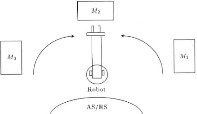
In order to explain the problem, consider a machining cell, where three-machine tools are located. A robot is used to feed these three machines, namely, M1,
M2 and M3, in the cell, where parts are brought to
and removed from the robotic cell by an Automated Storage & Retrieval System (AS/RS). The pallets and feeders of the AS/RS system allow hundreds of parts to be loaded into the cell without human intervention (see Figure 1) and the machines can be congured to perform any operation. The aim of this paper is to nd a schedule for the robot movement and the sequence of parts to maximize throughput (i.e., to minimize cycle time).
In each cycle, n parts (the total number of parts in the MPS) are produced, in which r1 are the parts
of part type 1 and r2 are the parts of part type 2.
In an m-machine exible cell, all parts in a MPS visit each machine in the same order. However, the operations can be performed in any order and each machine can be congured to perform any opera-tion.
Sethi et al. [6] showed that there are exactly m! potentially optimal 1-unit cycles in a m-machine ow-shop robotic cell (note that a 1-unit cycle returns to the same state after the production of a single unit). They also showed that any potentially optimal 1-unit robot move cycle in a m-machine robotic cell can be described by exactly m + 1, following basic activities:
Mi : Load a part on Mi; i = 1; 2; m;
M+
m: Unload a nished part from Mm:
Note that, in a 1-unit cycle, every basic activity must be carried out exactly once. Moreover, since, in an optimal cycle we require that the robot move path
be as short as possible, any two consecutive activities uniquely determine the robot moves between them. Therefore, a cycle can be uniquely described by a permutation of the above m + 1 activities. The following are the available robot move cycles for a m = 3 ow-shop robotic cell, as described by Sethi et al. [6]:
S1: fM+
3 ; M1; M2; M3 ; M3+g;
S2: fM+
3 ; M1; M3; M2 ; M3+g;
S3: fM+
3 ; M3; M1; M2 ; M3+g;
S4: fM+
3 ; M2; M3; M1 ; M3+g;
S5: fM+
3 ; M2; M1; M3 ; M3+g;
S6: fM+
3 ; M3; M2; M1 ; M3+g:
In ow-shop robotic cells, the computational results obtained by Hall et al. [3] suggest that, besides their practical advantages, 1-unit robot move cycles rou-tinely provide schedules with cycle times that are very close to the lower bounds available for all possible robot move cycles.
Lemma 1
For the exible robotic cell there are (m!)2 potentially
optimal 1-unit cycles. Proof
From Sethi et al. [6] we have m! potential optimal 1-unit cycles in a m machine ow-shop. For every poten-tially optimal cycle sequence of a ow-shop robotic cell, we have a m machine arranged as M1; M2; ; Mm.
To produce a exible robotic cell, we can rearrange the operations of every ow-shop robotic cell by m! possible arrangements. Thus, we have (m!)2potentially optimal
1-unit cycles in exible robotic cells and this completes the proof.
The category number is described as the super-script on the policy notations, i.e., Sk represents policy
S under category k. Similar notations are also used for cycle times, T .
Category 1
Under this category, six possible move cycles for an open-shop problem are dened. The move cycle, S1
I, is
similar to S1 in the three-machine ow-shop problem
described by Sethi et al. [6], and the problem of nding the best part sequence to be processed using the robot move cycle, S1, is solved trivially [3].
Lemma 2
The cycle time of one unit, for the policies under Category 1, are given by:
T1
I;(i)= ^TI;(i)1 = TII;()1 = ^TII;()1 = TIII;()1
= ^T1
III;()= a(i)+ b(i)+ c(i)+ 8" + 4:
Proof
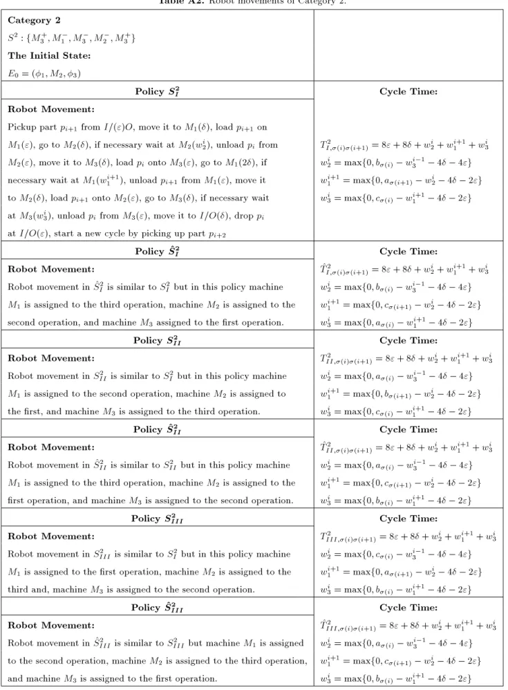
Refer to the Appendix, Table A1. Category 2
Under this category, six possible move cycles for a ex-ible robotic cell problem are dened. The move cycle, S2
I, is similar to S2 in the three-machine ow-shop
problem described by Sethi et al. [6] and the problem of nding the best part sequence to be processed, using the robot move cycle, S2, is NP-Complete [4].
Lemma 3
The cycle times of one unit for the policies under Category 2 are given by:
T2
I;(i)(i+1)= 8" + 8 + maxf0; c(i) 4
2"; a(i+1) 4 2"; a(i)
+ b(i);a(i+1)+ b(i+1)2 + c(i+1)
6 4"g; ^
T2
I;(i)(i+1)= 8" + 8 + maxf0; a(i) 4
2"; c(i+1) 4 2"; c(i)
+ b(i);a(i+1)+ b(i+1)2 + c(i+1)
6 4"g; T2
II;(i)(i+1)= 8" + 8 + maxf0; c(i) 4
2"; b(i+1) 4 2"; a(i)
+ b(i);a(i+1)+ b(i+1)2 + c(i+1)
6 4"g; ^
T2
II;(i)(i+1)= 8" + 8 + maxf0; b(i) 4
+ c(i);a(i+1)+ b(i+1)2 + c(i+1)
6 4"g; T2
III;(i)(i+1)= 8" + 8 + maxf0; b(i) 4
2"; a(i+1) 4 2"; a(i)
+ c(i);a(i+1)+ b(i+1)2 + c(i+1)
6 4"g; ^
T2
III;(i)(i+1)= 8" + 8 + maxf0; a(i) 4
2"; b(i+1) 4 2"; b(i)
+c(i);a(i+1)+ b(i+1)2 + c(i+1)
6 4"g: Proof
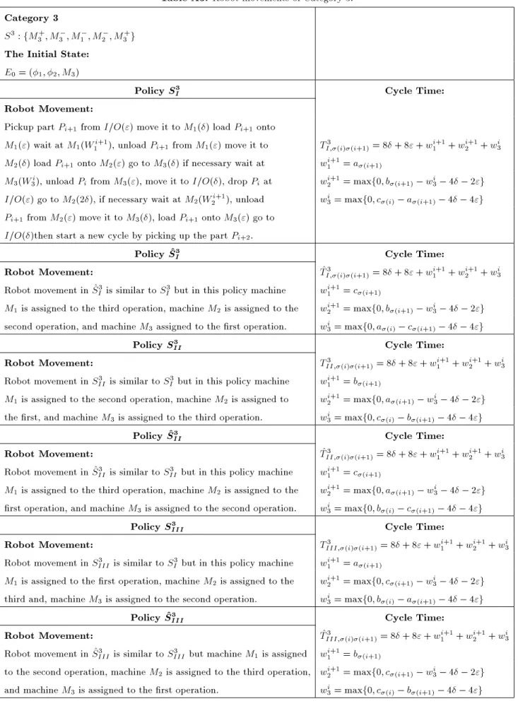
Refer to the Appendix, Table A2. Category 3
Under this category, six possible move cycles for a exible robotic cell problem are dened. The move cycle, s3
I, is similar to S3in the three-machine ow-shop
problem described by Sethi et al. [6] and the problem of nding the best part sequence to be processed using the robot move cycle, S3, can be solved optimally in
O(n log n) time [3]. Lemma 4
The cycle times of one unit for the policies under Category 3 are given by:
T3
I;(i)(i+1)= 8 + 8" + maxfa(i+1); c(i) 4
4"; a(i+1)+ b(i+1) 4 2"g;
^ T3
I;(i)(i+1)= 8 + 8" + maxfc(i+1); a(i) 4
4"; c(i+1)+ b(i+1) 4 2"g;
T3
II;(i)(i+1)= 8 + 8" + maxfb(i+1); c(i) 4
4"; a(i+1)+ b(i+1) 4 2"g;
^ T3
II;(i)(i+1)= 8 + 8" + maxfc(i+1); b(i) 4
4"; a(i+1)+ c(i+1) 4 2"g;
T3
III;(i)(i+1)= 8 + 8" + maxfa(i+1); b(i) 4
4"; a(i+1)+ c(i+1) 4 2"g;
^ T3
III;(i)(i+1)= 8 + 8" + maxfb(i+1); c(i) 4
4"; b(i+1)+ c(i+1) 4 2"g:
Proof
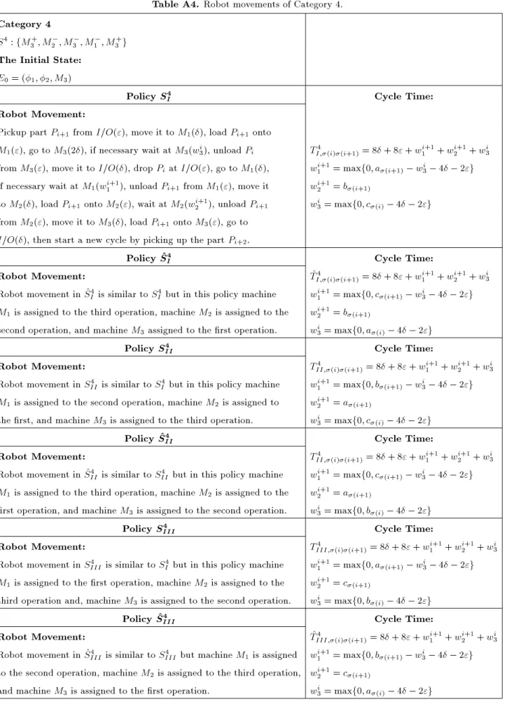
Refer to the Appendix, Table A3. Category 4
Under this category, six possible move cycles for an open-shop problem are dened. The move cycle, S4
I, is
similar to S4 in the three-machine ow-shop problem
described by [6] and the problem of nding the best part sequence to be processed, using the robot move cycle S4, can be solved optimally in On log(n) time [3].
Lemma 5
The cycle times of one unit for the policies under Category 4 are given by:
T4
I;(i)(i+1)= 8 + 8" + maxfb(i+1); b(i+1)+ c(i)
4 2"; a(i+1)+ b(i+1) 4 2"g;
^ T4
I;(i)(i+1)= 8 + 8" + maxfb(i+1); b(i+1)+ a(i)
4 2"; b(i+1)+ c(i+1) 4 2"g;
T4
II;(i)(i+1)=8+8"+maxfa(i+1); a(i+1)+c(i)
4 2"; a(i+1)+ b(i+1) 4 2"g;
^ T4
II;(i)(i+1)=8+8"+maxfa(i+1); a(i+1)+b(i)
4 2"; a(i+1)+ c(i+1) 4 2"g;
T4
III;(i)(i+1)=8+8"+maxfc(i+1); b(i+1)+c(i)
4 2"; a(i+1)+c(i+1) 4 2"g;
^ T4
III;(i)(i+1)=8+8"+maxfc(i+1); c(i+1)+a(i)
4 2"; b(i+1)+ c(i+1) 4 2"g:
Proof
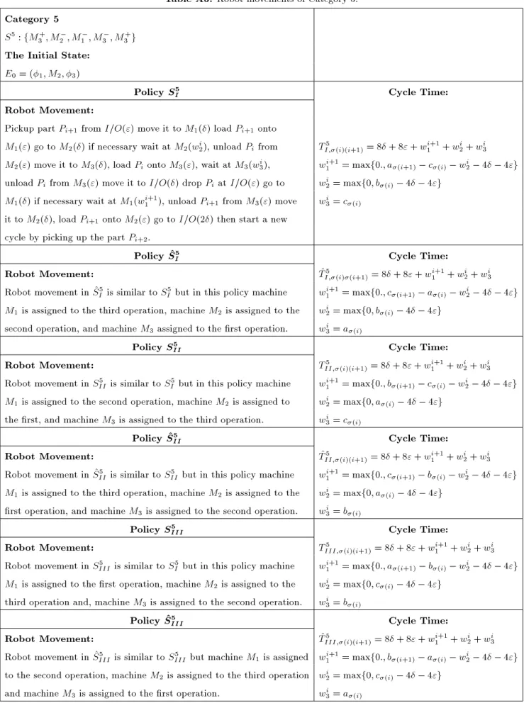
Category 5
Under this category, six possible move cycles for an open-shop problem are dened. The move cycle, S5
I, is
similar to S5 in the three-machine ow-shop problem
described by Sethi et al. [6] and the problem of nding the best part sequence to be processed, using the robot move cycle S5, can be solved optimally in On log(n)
time [3]. Lemma 6
The cycle times of one unit for the policies under Category 5 are given by:
T5
I;(i)(i+1)= 8 + 8" + maxfc(i); b(i)+ c(i) 4
2"; a(i+1) 4 4"g;
^ T5
I;(i)(i+1)= 8 + 8" + maxfa(i); a(i)+ b(i) 4
2"; c(i+1) 4 4"g;
T5
II;(i)(i+1)= 8 + 8" + maxfc(i); a(i)+ c(i) 4
2"; b(i+1) 4 4"g;
^ T5
II;(i)(i+1)= 8 + 8" + maxfb(i); a(i)+ b(i) 4
2"; c(i+1) 4 4"g;
T5
III;(i)(i+1)= 8 + 8" + maxfb(i); b(i)+ c(i) 4
2"; a(i+1) 4 4"g;
^ T5
III;(i)(i+1)= 8 + 8" + maxfa(i); a(i)+ c(i) 4
2"; b(i+1) 4 4"g:
Proof
Refer to the Appendix, Table A5. Category 6
Under this category, six possible move cycles for an open-shop problem are dened. The move cycle, S6
I, is
similar to S6 in the three-machine ow-shop problem
described by Sethi et al. [6] and the problem of nding the best part sequence to be processed, using the robot move cycle S6, is NP-complete [4].
Lemma 7
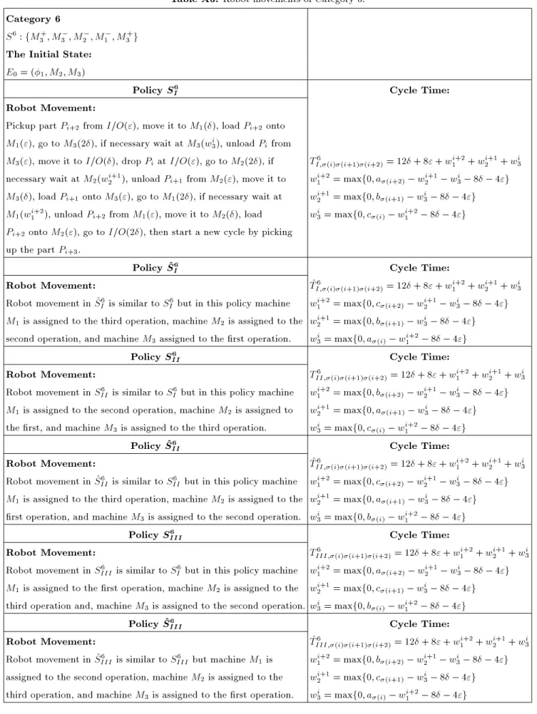
The cycle times of one unit for the policies under Category 6 are given by:
T6
I;(i)(i+1)(i+2)= 12 + 8" + maxf0; a(i+2) 8
4"; b(i+1) 8 4"; c(i) 8 4"g;
^ T6
I;(i)(i+1)(i+2)= 12 + 8" + maxf0; c(i+2) 8
4"; b(i+1) 8 4"; a(i) 8 4"g;
T6
II;(i)(i+1)(i+2)= 12 + 8" + maxf0; b(i+2) 8
4"; a(i+1) 8 4"; c(i) 8 4"g;
^ T6
II;(i)(i+1)(i+2)= 12 + 8" + maxf0; c(i+2) 8
4"; a(i+1) 8 4"; b(i) 8 4"g;
T6
III;(i)(i+1)(i+2)= 12 + 8" + maxf0; a(i+2) 8
4"; c(i+1) 8 4"; b(i) 8 4"g;
^ T6
III;(i)(i+1)(i+2)= 12 + 8" + maxf0; b(i+2) 8
4"; c(i+1) 8 4"; a(i) 8 4"g:
Proof
Refer to the Appendix, Table A6.
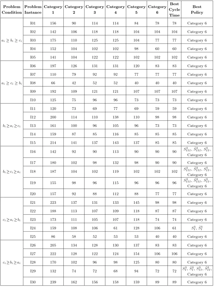
The computational results of Lemmas 2-7 are shown in Table A7. For the experiments, we considered that the values of " and are equal to 1; the processing times for all parts on all machines are uniformly generated in the range [10,100] and the parts are identical.
Theorem 1
If in a three-machine robotic cell with identical parts the processing times on all three machines are larger than, or equal to, 8 + 4", and the operations are arranged in such a way that the longest operation is assigned to machine M1, the shortest operation
is assigned to machine M3 and the last operation is
assigned to machine M2, the policies under Category 6
will have the minimum cycle time. Proof
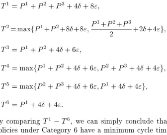
First, consider the following notations: p1= maxfa; b; cg; P3= minfa; b; cg;
According to Lemmas 2 to 7, the cycle time of dierent policies in this case will be as follows:
T1= P1+ P2+ P3+ 4 + 8";
T2=maxfP1+P2+8+8";P1+P2+P3
2 +2+4"g; T3= P1+ P2+ 4 + 6";
T4= maxfP1+ P2+ 4 + 6"; P2+ P3+ 4 + 4"g;
T5= maxfP2+ P3+ 4 + 6"; P1+ 4 + 4"g;
T6= P1+ 4 + 4":
By comparing T1 T6, we can simply conclude that
policies under Category 6 have a minimum cycle time and the proof will be complete.
From here, we will consider policy S6 I.
DEVELOPING THE MATHEMATICAL MODELS
In this section, we develop a systematic method to produce the necessary mathematical programming for-mulation for robotic cells. Therefore, rst, we model a single-part type problem using Petri-nets and, then, we adapt the mathematical programming approach to the problem. Second, we extend the model to a multiple-part type problem.
Single-Part Type Problem ORC3jk = 1, SI6jCt
Without loss of generality in the modeling approach, the movements of the robot arm will be restricted to
policy S6
I, as shown in Figure 2. The robot arm, at
steady state, is located at machine M2, therefore, by
coming back to this node, we have a complete cycle for the robot arm. This policy is described in Figure 2. For further formulation of the problem, we need to dene the Petri-nets and their related characteristics.
A Petri-net is a quadruple, P N(P; T; A; W ), where P = fp1; p2; ; png is a nite set of places,
T = ft1; t2; ; tmg is a nite set of transitions,
A (P T ) [ (T P ) is a nite set of arcs and W : A ! f1; 2; 3; g is a weight function. Every place has an initial marking, M0 : P ! f0; 1; 2; g.
If we assign time to the transitions, we call it a timed Petri-net.
The behavior of many systems can be described by system states and their changes, in order to simulate the dynamic behavior of the system. The marking in a Petri-net is changed, according to the following transition (ring) rule:
1. A transition is said to be enabled, if each input place, p of t, is marked at least with w(p; t) tokens, where w(p; t) is the weight of the arc from p to t; 2. An enabled transition may or may not be red
(depending on whether or not the event takes place);
3. The ring of an enabled transition, t, removes w(p; t) tokens from each input place, p of t, and adds w(t; p) tokens to each output place, p of t, where w(t; p) is the weight of the arc from t to p.
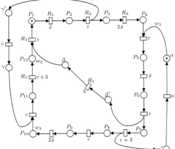
The related timed Petri-net for robot movements under policy S6
I is shown in Figure 3. All the weights
of the arcs are constant and can be ignored. The descriptions of the transitions for this graph, with respective execution times, would be as follows:
Figure 2. the robot movement in three-machine robotic cell under policy S6 I.
Figure 3. Petri net; presentation of policy S6 I under
Category 6.
R1: go to M3();
R2: load M3(");
R3: go to M1(2);
RP1: wait at M1(wi1);
R4: unload M1(");
R5: go to M2(2);
R6: Load M2(");
R7: go to input, pickup a new part, move it to
M1(" + 3);
R8: load M1(");
R9: go to M3(2);
RP3: wait at M3(wi3);
R10: unload M3(");
R11: go to output, drop the part, go to M2("+3);
RP2: wait at M2(wi2);
R12: unload M2(");
in which the execution times are as follows: si: Starting time of operating transition Ri;
where i = 1; 2; ; 12;
spj : Starting time of operating transition RPj;
where j = 1; 2; 3;
The constraints of three machines process times are as follows:
: Machine M1 has processed the job and is readyto
be unloaded;
: Machine M2has processed the job and is ready to
be unloaded;
: Machine M3has processed the job and is ready to
be unloaded. Denition
A marked graph is a Petri-net, such that every place has only one input and only one output.
Theorem 2
For a marked graph, wherein every place has mitokens
(see Figure 4), the following relation, SB SA+miCt,
where SA, SB are the starting times of transitions A
and B, respectively, and \Ctis the cycle time", is true.
Proof: See [14].
For guaranteeing the liveness of the Petri-net, at the beginning, we put one token in place p1and one token
in place . During the production cycle, the tokens are moving to dierent places and, after completion of a cycle, the tokens are replaced at the same beginning places; thereafter, another cycle can be repeated. Since the Petri-net model of the problem is a marked graph, based on Theorem 2, the following linear programming
can be developed. min C6
t;
subject to :
p1: s1 s12+ Ct6= "; (1)
p2: s2 s1= ; (2)
P3: s3 s2= "; (3)
P P1: sp1 s3= 2; (4)
p4: s4 sp1 w1= 0; (5)
P5: s5 s4= "; (6)
P6: s6 s5= ; (7)
p7: s7 s6= "; (8)
P8: s8 s7= " + 3; (9)
P9: s9 s8= "; (10)
P P3: sp3 s9= 2; (11)
P10: s10 sp3 w3= 0; (12)
P11: s11 s10= "; (13)
P P2: sp2 s11= " + 3; (14)
P12: s12 sp2 w2= 0; (15)
: s4 s7+ Ct6 a + "; (16)
: s12 s6 b + "; (17)
: s10 s2 c + "; (18)
si 0; i = 1; 2; ; 12; spj 0; i = 1; 2; 3;
wj 0; j = 0; 1; 2; 3:
Notice that, to avoid the deadlock in the steady state, it is assumed that machine M1has processed its job and
is waiting for the robot, where machines M2 and M3
are in an idle status and the robot arm is moving one part to machine M3. The above formulation has some
signicant advantages over the previous model. First, it is simply a network problem that has polynomial time complexity and, second, it computes the starting times for every status of robot movement, which is more convenient than computing the waiting times of the robot arm.
Multi-Part Type Systems, ORC3jk 2, SI6jCt
The single part type problem is not a very complicated problem. In this section, a system that allows a multiple part type will be studied. For example, at machine M1, when we want to load a part on the
machine, we have to decide which part should be chosen, such that the cycle time is minimized. The same thing can also be achieved for M2and M3. Based
on the choosing gate denition [15], we simply have three choosing gates, as , and . Thus, we can write the following formulations using 0-1 integer variables, x1ij, x2ij and x3ij, as:
1: s4;1 s8;n+ Ct= n
X
i=1
x1in(ai+ 'i) + ";
j : s4;j+1 s8;j = n
X
i=1
x1ij(ai+ 'i) + ";
j = 2; ; n; j : s12;j s6;j =
n
X
i=1
x2ij(bi+ 'i) + ";
j = 1; ; n; j : s10;j s2;j =
n
X
i=1
x3ij(ci+ 'i) + ";
j = 1; ; n:
In addition, the following feasibility constraints assign a unique positioning for every job:
n
X
i=1
x1ij= 1; j = 1; ; n;
n
X
j=1
x1ij= 1; i = 1; ; n:
To keep the sequence of the parts between the machines in the correct order, we have to add the following constraints:
x1i;j= x2i;j+1; i = 1; ; n; j = 1; ; n;
x2i;j= x3i;j+1; i = 1; ; n; j = 1; ; n;
where it is assumed that x1i;n+1 = x1i;1, because of
the cyclic repetition of parts.
Thus, the complete model for the three-machine robotic cells with multiple-parts would be as follows:
min C6 t;
subject to :
p1;1 : s2;1 s12;n+ Ct= " + ;
j = 2; ; n; (19)
p1;j : s2j s12j = " + ;
j = 1; ; n; (20)
p3;j : s4j s2j w1j = " + 2;
j = 1; ; n; (21)
p5;j : s6j s4j = " + ;
j = 1; ; n; (22)
p7;j : s8j s6j = 2" + 3;
j = 1; ; n; (23)
p9;j : s10j s8j w3j = " + 2;
j = 1; ; n; (24)
p11;j : s12j s10j w2j=2"+3;
j = 1; ; n; (25)
1: s4;1 s7;1+ Ct n
X
i=1
x1in(ai+ 'ai) "; (26)
j : s4;j s7;j n
X
i=1
x1ij(ai+ 'ai) ";
j = 2; ; n; (27)
j : s12;j s6;j n
X
i=1
x2ij(bi+ 'bi) ";
j = 1; ; n; (28)
j: s10;j s2;j n
X
i=1
x3ij(ci+ 'ci) ";
j = 1; ; n; (29)
x1i;j 1= x2i;j; i; j = 1; ; n; (30)
x2i;j 1= x3i;j; i; j = 1; ; n; (31) n
X
i=1
x1ij = 1; j = 1; ; n; (32)
n
X
j=1
x1ij = 1; i = 1; ; n; (33)
si;j 0; i = 1; ; 12; j = 1; 2; ; n;
wkj 0; k = 0; 1; 2; 3; j = 1; ; n;
x1; x2; x3 2 f0; 1g:
This mathematical model can be developed for other policies under Category 6. These models are coded into lingo 8 and run on the Core (TM) 2 Due T7100 processor at 1.8 GHz and Windows vista, using 2 GB of RAM. For the experiments, we consider the values of " and as being equal to 1; the processing times for all parts on all machines are uniformly generated in the range [10, 100].
The problem instances are randomly generated as Table A8.
SOLUTION ALGORITHMS
In a single-part type problem, the parts, which are produced in a cell, are identical. Thus, it is necessary to consider only robot movements to produce the best solution for the problem. In a multiple-part type robotic cell, the formation of MPS is dened, according to the market demand of dierent products. Therefore, two decisions need to be made: (a) Choosing a robot move sequence and (b) Determining a part sequence. In practice, the MPS can be larger than 50 parts, thus, the sequence of parts in a robotic cell is very important. According to the Sriskandarajah classication scheme [5], for the complexity of this robotic cell scheduling problem, scheduling problems of policies under Category 1 are sequence indepen-dent and are trivially solvable (they are U-class [5]). Scheduling problems of policies under Categories 3, 4 and 5 can be modeled as the special case of a travelling salesman problem, which is solvable in polynomial time by the Glimor and Gomary algorithm [16] (they are V 1-class [5]). Scheduling problems of policies under Categories 2 and 6 are NP-Complete (they are W-class [5]). The mathematical model introduced in Section 5 can be used for medium size problems, but, further research is needed to introduce heuristics or meta-heuristics in the solving of large size problems. Baghchi [17] proposed an algorithm to solve m-machine cells. By using this algorithm, the sequence of parts in a MPS and robot movement policy that minimizes the 1-unit cycle time, is obtained. This algorithm is as follows:
Step 1 Let Tu denotes the minimum cycle time of a
Step 2 Use the algorithm of Gilmore and Gomory to solve the part sequencing problem for all policies in a V 1-class. Let Tv1 denote the
minimum cycle time in the V 1-class;
Step 3 Use a mathematical model (for small size prob-lems) or a heuristic (for large size probprob-lems) to solve the part sequencing problems for all policies in a W -class. Let Tw denote the
minimum cycle time among W -cycles;
Step 4 Find Th = minfTu; Tv1; Tv2; Twg and its
asso-ciated policy and part sequence. Terminate. CONCLUSION
In this paper, we consider a manufacturing cell, in which a robot loads/ unloads machines and moves parts between machines. In this robotic cell, machines are exible and are able to do all operations that are necessary for producing all parts. The robotic cell may produce dierent part types and each part consists of three operations. In this paper, we recognize thirty six potential optimal 1-unit cycles by consider-ing operational exibility and the policies that have been introduced by Sethi et al. [6]. Twelve policies, which are under categories S2 and S6, are Unary
NP-complete. We introduce formulas for calculating the cycle time of thirty six policies when the sequences of parts are given. The formulas achieved by considering the waiting times of a robot for unloading a completed part from machines M1, M2, and M3, and under the
condition that one of the categories (i.e. S6) had the
minimum cycle time, were identied.
In this paper, a mathematical model using Petri-nets was proposed, to nd the parts sequence and robot movements that minimize the cycle time (i.e. maximize throughput). This model has signicant advantages over previous model formulations. Based on the single model formulation, a general mathematical model was developed for a multi-part type problem. Finally, an algorithm is introduced to solve this problem. In further works to appear soon, we implemented other issues, such as a no-wait robot environment.
REFERENCES
1. Asfahl, C.R., Robots and Manufacturing Automation, 2nd Ed., New York, John Wiley and Sons (1992). 2. Crama, Y. et al. \Cyclic scheduling in robotic ow
shops", Annals of Operations Research, 96, pp. 97-124 (2000).
3. Hall, N.G., Kamoun, H. and Sriskandarajah, C. \Scheduling in robotic cells: Classication, two and three machine cells", Operations Research, 45(2), pp. 421-439 (1997).
4. Hall, N.G., Kamoun, H. and Sriskandarajah, C. \Scheduling in robotic cells: complexity and steady
state analysis", European Journal of Operational Re-search, 109, pp. 43-65 (1998).
5. Sriskandarajah, C. et al. \Scheduling large robotic cells without buers", Annals of Operations Research, 76, pp. 287-321 (1998).
6. Sethi, S.P. et al. \Sequencing of parts and robot moves in a robotic cell", International Journal of Flexible Manufacturing Systems, 4, pp. 331-358 (1992). 7. Blazewicz, J., Sethi, S.P. and Sriskandarajah, C.
\Scheduling of robot moves and parts in a robotic cell", in Third ORSA/TIMS Conference on Flexible Man-ufacturing Systems: Operations Research Models and Applications, Amsterdam, The Netherlands, Elsevier Science Publishers (1989).
8. Crama, Y. and Klundert, V.D. \Cyclic scheduling in 3-machine robotic ow shops", Journal of Scheduling, 2, pp. 35-54 (1999).
9. Brauner, N. and Finke, G. \On a conjecture about robotic cells: New simplied proof for the three-machine case", INFOR, 37(1), pp. 20-36 (1999). 10. Dawande, M, et al. \Sequencing and Scheduling in
Robotic Cells: Recent Developments", Journal of Scheduling, 8, pp. 387-426 (2005).
11. Gultekin, H., Akturk, M.S. and Karasan, O.E. \Cyclic scheduling of a 2-machine robotic cell with tooling con-straints", European Journal of Operational Research, 174, pp. 777-796 (2006).
12. Gultekin, H., Akturk, M.S. and Karasan, O.E. \Scheduling in a three-machine robotic exible manu-facturing cell", Computers & Operations Research, 34, pp. 2463-2477 (2007).
13. Geismar, H.N., Dawande, M. and Sriskandarajah, C. \Approximation algorithms for k-unit cyclic solutions in robotic cells", European Journal of Operational Research, 162, pp. 291-309 (2005).
14. Maggot, J. \Performance evaluation of concurrent systems using Petri-nets", Inform. Processing Lett., 18(1), pp. 7-13 (1984).
15. Abadi, I.N.K. \A new formulation for scheduling prob-lems through Petri-nets", in the Iranian Mathematical Conference, Tabriz, Iran (1996).
16. Gilmore, P. and Gomory, R. \Sequencing a one-state variable machine: A solvable case of the traveling salesman problem", Operations Research, 12, pp. 675-679 (1964).
17. Bagchi, T.P., Gupta, J.N.D. and Sriskandarajah, C., \A review of TSP based approaches for ow shop scheduling", European Journal of Operational Research, 169, pp. 816-854 (2006).
APPENDIX
The waiting times relating to Lemmas 2 to 7 are calculated, based on the Petri-nets of each policy, and cycle times are calculated in the following tables.
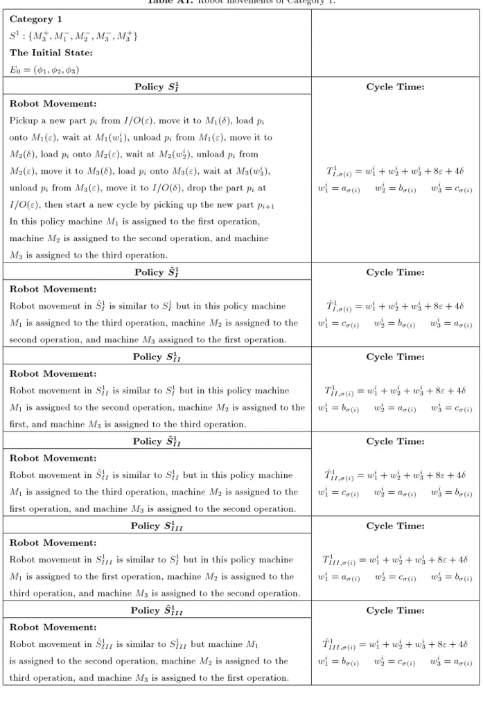
Table A1. Robot movements of Category 1. Category 1
S1: fM+
3; M1; M2 ; M3 ; M3+g
The Initial State: E0= (1; 2; 3)
Policy S1
I Cycle Time:
Robot Movement:
Pickup a new part pi from I=O("), move it to M1(), load pi
onto M1("), wait at M1(wi1), unload pifrom M1("), move it to
M2(), load pionto M2("), wait at M2(w2i), unload pifrom
M2("), move it to M3(), load pi onto M3("), wait at M3(wi3), TI;(i)1 = wi1+ wi2+ wi3+ 8" + 4
unload pifrom M3("), move it to I=O(), drop the part piat wi1= a(i) wi2= b(i) wi3= c(i)
I=O("), then start a new cycle by picking up the new part pi+1
In this policy machine M1 is assigned to the rst operation,
machine M2 is assigned to the second operation, and machine
M3 is assigned to the third operation.
Policy ^S1
I Cycle Time:
Robot Movement: Robot movement in ^S1
I is similar to SI1 but in this policy machine T^I;(i)1 = wi1+ wi2+ wi3+ 8" + 4
M1 is assigned to the third operation, machine M2is assigned to the wi1= c(i) wi2= b(i) wi3= a(i)
second operation, and machine M3 assigned to the rst operation.
Policy S1
II Cycle Time:
Robot Movement: Robot movement in S1
II is similar to SI1 but in this policy machine TII;(i)1 = wi1+ wi2+ wi3+ 8" + 4
M1 is assigned to the second operation, machine M2is assigned to the wi1= b(i) wi2= a(i) wi3= c(i)
rst, and machine M3 is assigned to the third operation.
Policy ^S1
II Cycle Time:
Robot Movement: Robot movement in ^S1
II is similar to SII1 but in this policy machine T^II;(i)1 = wi1+ wi2+ wi3+ 8" + 4
M1 is assigned to the third operation, machine M2is assigned to the wi1= c(i) wi2= a(i) w3i= b(i)
rst operation, and machine M3 is assigned to the second operation.
Policy S1
III Cycle Time:
Robot Movement: Robot movement in S1
III is similar to SI1but in this policy machine TIII;(i)1 = wi1+ wi2+ wi3+ 8" + 4
M1 is assigned to the rst operation, machine M2is assigned to the wi1= a(i) wi2= c(i) w3i= b(i)
third operation, and machine M3 is assigned to the second operation.
Policy ^S1
III Cycle Time:
Robot Movement: Robot movement in ^S1
III is similar to SIII1 but machine M1 T^III;(i)1 = wi1+ wi2+ wi3+ 8" + 4
is assigned to the second operation, machine M2 is assigned to the wi1= b(i) wi2= c(i) wi3= a(i)
Table A2. Robot movements of Category 2. Category 2
S2: fM+
3; M1 ; M3 ; M2; M3+g
The Initial State: E0= (1; M2; 3)
Policy S2
I Cycle Time:
Robot Movement:
Pickup part pi+1from I=(")O, move it to M1(), load pi+1on
M1("), go to M2(), if necessary wait at M2(wi2), unload pifrom TI;(i)(i+1)2 = 8" + 8 + wi2+ wi+11 + wi3
M2("), move it to M3(), load pi onto M3("), go to M1(2), if w2i= maxf0; b(i) wi 13 4 4"g
necessary wait at M1(wi+11 ), unload pi+1from M1("), move it w1i+1= maxf0; a(i+1) wi2 4 2"g
to M2(), load pi+1onto M2("), go to M3(), if necessary wait w3i= maxf0; c(i) wi+11 4 2"g
at M3(w3i), unload pifrom M3("), move it to I=O(), drop pi
at I=O("), start a new cycle by picking up part pi+2
Policy ^S2
I Cycle Time:
Robot Movement: T^2
I;(i)(i+1)= 8" + 8 + wi2+ wi+11 + wi3
Robot movement in ^S2
I is similar to SI2 but in this policy machine w2i= maxf0; b(i) wi 13 4 4"g
M1 is assigned to the third operation, machine M2 is assigned to the w1i+1= maxf0; c(i+1) w2i 4 2"g
second operation, and machine M3 assigned to the rst operation. w3i= maxf0; a(i) wi+11 4 2"g
Policy S2
II Cycle Time:
Robot Movement: T2
II;(i)(i+1)= 8" + 8 + w2i+ w1i+1+ w3i
Robot movement in S2
II is similar to SI2 but in this policy machine w2i= maxf0; a(i) wi 13 4 4"g
M1 is assigned to the second operation, machine M2 is assigned to w1i+1= maxf0; b(i+1) wi2 4 2"g
the rst, and machine M3 is assigned to the third operation. w3i= maxf0; c(i) wi+11 4 2"g
Policy ^S2
II Cycle Time:
Robot Movement: T^2
II;(i)(i+1)= 8" + 8 + w2i+ w1i+1+ w3i
Robot movement in ^S2
II is similar to SII2 but in this policy machine w2i= maxf0; a(i) wi 13 4 4"g
M1 is assigned to the third operation, machine M2 is assigned to the w1i+1= maxf0; c(i+1) w2i 4 2"g
rst operation, and machine M3 is assigned to the second operation. w3i= maxf0; b(i) wi+11 4 2"g
Policy S2
III Cycle Time:
Robot Movement: T2
III;(i)(i+1)= 8" + 8 + wi2+ wi+11 + wi3
Robot movement in S2
III is similar to SI2 but in this policy machine w2i= maxf0; c(i) wi 13 4 4"g
M1 is assigned to the rst operation, machine M2 is assigned to the w1i+1= maxf0; a(i+1) wi2 4 2"g
third and, machine M3 is assigned to the second operation. w3i= maxf0; b(i) wi+11 4 2"g
Policy ^S2
III Cycle Time:
Robot Movement: T^2
III;(i)(i+1)= 8" + 8 + wi2+ wi+11 + wi3
Robot movement in ^S2
III is similar to SIII2 but machine M1 is assigned w2i= maxf0; a(i) wi 13 4 4"g
to the second operation, machine M2 is assigned to the third operation, w1i+1= maxf0; c(i+1) w2i 4 2"g
Table A3. Robot movements of Category 3. Category 3
S3: fM+
3 ; M3 ; M1 ; M2 ; M3+g
The Initial State: E0= (1; 2; M3)
Policy S3
I Cycle Time:
Robot Movement:
Pickup part Pi+1from I=O(") move it to M1() load Pi+1onto
M1(") wait at M1(W1i+1), unload Pi+1from M1(") move it to TI;(i)(i+1)3 = 8 + 8" + wi+11 + wi+12 + wi3
M2() load Pi+1 onto M2(") go to M3() if necessary wait at wi+11 = a(i+1)
M3(W3i), unload Pifrom M3("), move it to I=O(), drop Pi at wi+12 = maxf0; b(i+1) w3i 4 2"g
I=O(") go to M2(2), if necessary wait at M2(W2i+1), unload wi3= maxf0; c(i) a(i+1) 4 4"g
Pi+1from M2(") move it to M3(), load Pi+1onto M3(") go to
I=O()then start a new cycle by picking up the part Pi+2.
Policy ^S3
I Cycle Time:
Robot Movement: T^3
I;(i)(i+1)= 8 + 8" + wi+11 + wi+12 + wi3
Robot movement in ^S3
I is similar to SI3 but in this policy machine wi+11 = c(i+1)
M1is assigned to the third operation, machine M2 is assigned to the wi+12 = maxf0; b(i+1) w3i 4 2"g
second operation, and machine M3 assigned to the rst operation. wi3= maxf0; a(i) c(i+1) 4 4"g
Policy S3
II Cycle Time:
Robot Movement: T3
II;(i)(i+1)= 8 + 8" + wi+11 + w2i+1+ w3i
Robot movement in S3
IIis similar to SI3 but in this policy machine wi+11 = b(i+1)
M1is assigned to the second operation, machine M2 is assigned to wi+12 = maxf0; a(i+1) wi3 4 2"g
the rst, and machine M3 is assigned to the third operation. wi3= maxf0; c(i) b(i+1) 4 4"g
Policy ^S3
II Cycle Time:
Robot Movement: T^3
II;(i)(i+1)= 8 + 8" + wi+11 + w2i+1+ w3i
Robot movement in ^S3
IIis similar to SII3 but in this policy machine wi+11 = c(i+1)
M1is assigned to the third operation, machine M2 is assigned to the wi+12 = maxf0; a(i+1) wi3 4 2"g
rst operation, and machine M3 is assigned to the second operation. wi3= maxf0; b(i) c(i+1) 4 4"g
Policy S3
III Cycle Time:
Robot Movement: T3
III;(i)(i+1)= 8 + 8" + w1i+1+ wi+12 + wi3
Robot movement in S3
III is similar to S3I but in this policy machine wi+11 = a(i+1)
M1is assigned to the rst operation, machine M2 is assigned to the wi+12 = maxf0; c(i+1) w3i 4 2"g
third and, machine M3 is assigned to the second operation. wi3= maxf0; b(i) a(i+1) 4 4"g
Policy ^S3
III Cycle Time:
Robot Movement: T^3
III;(i)(i+1)= 8 + 8" + w1i+1+ wi+12 + wi3
Robot movement in ^S3
III is similar to S3III but machine M1is assigned wi+11 = b(i+1)
to the second operation, machine M2 is assigned to the third operation, wi+12 = maxf0; c(i+1) w3i 4 2"g
Table A4. Robot movements of Category 4. Category 4
S4: fM+
3 ; M2 ; M3; M1 ; M3+g
The Initial State: E0= (1; 2; M3)
Policy S4
I Cycle Time:
Robot Movement:
Pickup part Pi+1from I=O("), move it to M1(), load Pi+1onto
M1("), go to M3(2), if necessary wait at M3(wi3), unload Pi TI;(i)(i+1)4 = 8 + 8" + wi+11 + wi+12 + w3i
from M3("), move it to I=O(), drop Piat I=O("), go to M1(), w1i+1= maxf0; a(i+1) w3i 4 2"g
if necessary wait at M1(wi+11 ), unload Pi+1from M1("), move it w2i+1= b(i+1)
to M2(), load Pi+1onto M2("), wait at M2(wi+12 ), unload Pi+1 w3i= maxf0; c(i) 4 2"g
from M2("), move it to M3(), load Pi+1 onto M3("), go to
I=O(), then start a new cycle by picking up the part Pi+2.
Policy ^S4
I Cycle Time:
Robot Movement: T^4
I;(i)(i+1)= 8 + 8" + wi+11 + wi+12 + w3i
Robot movement in ^S4
I is similar to SI4but in this policy machine w1i+1= maxf0; c(i+1) wi3 4 2"g
M1 is assigned to the third operation, machine M2 is assigned to the w2i+1= b(i+1)
second operation, and machine M3assigned to the rst operation. w3i= maxf0; a(i) 4 2"g
Policy S4
II Cycle Time:
Robot Movement: T4
II;(i)(i+1)= 8 + 8" + w1i+1+ w2i+1+ wi3
Robot movement in S4
IIis similar to SI4but in this policy machine w1i+1= maxf0; b(i+1) wi3 4 2"g
M1 is assigned to the second operation, machine M2 is assigned to w2i+1= a(i+1)
the rst, and machine M3 is assigned to the third operation. w3i= maxf0; c(i) 4 2"g
Policy ^S4
II Cycle Time:
Robot Movement: T4
II;(i)(i+1)= 8 + 8" + w1i+1+ w2i+1+ wi3
Robot movement in ^S4
IIis similar to SII4 but in this policy machine w1i+1= maxf0; c(i+1) wi3 4 2"g
M1 is assigned to the third operation, machine M2 is assigned to the w2i+1= a(i+1)
rst operation, and machine M3 is assigned to the second operation. w3i= maxf0; b(i) 4 2"g
Policy S4
III Cycle Time:
Robot Movement: T4
III;(i)(i+1)= 8 + 8" + wi+11 + wi+12 + wi3
Robot movement in S4
III is similar to SI4 but in this policy machine w1i+1= maxf0; a(i+1) w3i 4 2"g
M1 is assigned to the rst operation, machine M2 is assigned to the w2i+1= c(i+1)
third operation and, machine M3is assigned to the second operation. w3i= maxf0; b(i) 4 2"g
Policy ^S4
III Cycle Time:
Robot Movement: T^4
III;(i)(i+1)= 8 + 8" + wi+11 + wi+12 + wi3
Robot movement in ^S4
III is similar to SIII4 but machine M1 is assigned w1i+1= maxf0; b(i+1) wi3 4 2"g
to the second operation, machine M2 is assigned to the third operation, w2i+1= c(i+1)
Table A5. Robot movements of Category 5. Category 5
S5: fM+
3; M2 ; M1 ; M3 ; M3+g
The Initial State: E0= (1; M2; 3)
Policy S5
I Cycle Time:
Robot Movement:
Pickup part Pi+1 from I=O(") move it to M1() load Pi+1onto
M1(") go to M2() if necessary wait at M2(wi2), unload Pifrom TI;(i)(i+1)5 = 8 + 8" + wi+11 + w2i+ wi3
M2(") move it to M3(), load Pi onto M3("), wait at M3(w3i), wi+11 = maxf0:; a(i+1) c(i) wi2 4 4"g
unload Pifrom M3(") move it to I=O() drop Pi at I=O(") go to wi2= maxf0; b(i) 4 4"g
M1() if necessary wait at M1(wi+11 ), unload Pi+1from M3(") move wi3= c(i)
it to M2(), load Pi+1 onto M2(") go to I=O(2) then start a new
cycle by picking up the part Pi+2.
Policy ^S5
I Cycle Time:
Robot Movement: T^5
I;(i)(i+1)= 8 + 8" + w1i+1+ w2i+ w3i
Robot movement in ^S5
I is similar to SI5 but in this policy machine wi+11 = maxf0:; c(i+1) a(i) wi2 4 4"g
M1 is assigned to the third operation, machine M2is assigned to the wi2= maxf0; b(i) 4 4"g
second operation, and machine M3 assigned to the rst operation. wi3= a(i)
Policy S5
II Cycle Time:
Robot Movement: T5
II;(i)(i+1)= 8 + 8" + w1i+1+ wi2+ wi3
Robot movement in S5
II is similar to SI5 but in this policy machine wi+11 = maxf0:; b(i+1) c(i) wi2 4 4"g
M1 is assigned to the second operation, machine M2 is assigned to wi2= maxf0; a(i) 4 4"g
the rst, and machine M3 is assigned to the third operation. wi3= c(i)
Policy ^S5
II Cycle Time:
Robot Movement: T^5
II;(i)(i+1)= 8 + 8" + w1i+1+ wi2+ wi3
Robot movement in ^S5
II is similar to SII5 but in this policy machine wi+11 = maxf0:; c(i+1) b(i) wi2 4 4"g
M1 is assigned to the third operation, machine M2is assigned to the wi2= maxf0; a(i) 4 4"g
rst operation, and machine M3 is assigned to the second operation. wi3= b(i)
Policy S5
III Cycle Time:
Robot Movement: T5
III;(i)(i+1)= 8 + 8" + wi+11 + wi2+ wi3
Robot movement in S5
III is similar to SI5but in this policy machine wi+11 = maxf0:; a(i+1) b(i) wi2 4 4"g
M1 is assigned to the rst operation, machine M2is assigned to the wi2= maxf0; c(i) 4 4"g
third operation and, machine M3 is assigned to the second operation. wi3= b(i)
Policy ^S5
III Cycle Time:
Robot Movement: T^5
III;(i)(i+1)= 8 + 8" + wi+11 + wi2+ wi3
Robot movement in ^S5
III is similar to SIII5 but machine M1 is assigned w1i+1= maxf0:; b(i+1) a(i) wi2 4 4"g
to the second operation, machine M2 is assigned to the third operation wi2= maxf0; c(i) 4 4"g
Table A6. Robot movements of Category 6. Category 6
S6: fM+
3; M3; M2 ; M1 ; M3+g
The Initial State: E0 = (1; M2; M3)
Policy S6
I Cycle Time:
Robot Movement:
Pickup part Pi+2 from I=O("), move it to M1(), load Pi+2 onto
M1("), go to M3(2), if necessary wait at M3(w3i), unload Pi from
M3("), move it to I=O(), drop Piat I=O("), go to M2(2), if TI;(i)(i+1)(i+2)6 = 12 + 8" + w1i+2+ w2i+1+ wi3
necessary wait at M2(wi+12 ), unload Pi+1from M2("), move it to wi+21 = maxf0; a(i+2) wi+12 wi3 8 4"g
M3(), load Pi+1onto M3("), go to M1(2), if necessary wait at wi+12 = maxf0; b(i+1) w3i 8 4"g
M1(w1i+2), unload Pi+2from M1("), move it to M2(), load wi3= maxf0; c(i) wi+21 8 4"g
Pi+2onto M2("), go to I=O(2), then start a new cycle by picking
up the part Pi+3.
Policy ^S6
I Cycle Time:
Robot Movement: T^6
I;(i)(i+1)(i+2)= 12 + 8" + w1i+2+ w2i+1+ wi3
Robot movement in ^S6
I is similar to SI6 but in this policy machine wi+21 = maxf0; c(i+2) wi+12 w3i 8 4"g
M1is assigned to the third operation, machine M2is assigned to the wi+12 = maxf0; b(i+1) w3i 8 4"g
second operation, and machine M3 assigned to the rst operation. wi3= maxf0; a(i) w1i+2 8 4"g
Policy S6
II Cycle Time:
Robot Movement: T6
II;(i)(i+1)(i+2)= 12 + 8" + wi+21 + wi+12 + wi3
Robot movement in S6
II is similar to SI6 but in this policy machine wi+21 = maxf0; b(i+2) w2i+1 w3i 8 4"g
M1is assigned to the second operation, machine M2is assigned to wi+12 = maxf0; a(i+1) wi3 8 4"g
the rst, and machine M3 is assigned to the third operation. wi3= maxf0; c(i) wi+21 8 4"g
Policy ^S6
II Cycle Time:
Robot Movement: T^6
II;(i)(i+1)(i+2)= 12 + 8" + wi+21 + wi+12 + wi3
Robot movement in ^S6
II is similar to SII6 but in this policy machine wi+21 = maxf0; c(i+2) wi+12 w3i 8 4"g
M1is assigned to the third operation, machine M2is assigned to the wi+12 = maxf0; a(i+1) wi3 8 4"g
rst operation, and machine M3 is assigned to the second operation. wi3= maxf0; b(i) wi+21 8 4"g
Policy S6
III Cycle Time:
Robot Movement: T6
III;(i)(i+1)(i+2)= 12 + 8" + wi+21 + w2i+1+ wi3
Robot movement in S6
III is similar to SI6but in this policy machine wi+21 = maxf0; a(i+2) wi+12 wi3 8 4"g
M1is assigned to the rst operation, machine M2is assigned to the wi+12 = maxf0; c(i+1) wi3 8 4"g
third operation and, machine M3 is assigned to the second operation. wi3= maxf0; b(i) wi+21 8 4"g
Policy ^S6
III Cycle Time:
Robot Movement: T^6
III;(i)(i+1)(i+2)= 12 + 8" + wi+21 + w2i+1+ wi3
Robot movement in ^S6
III is similar to SIII6 but machine M1 is w1i+2= maxf0; b(i+2) w2i+1 w3i 8 4"g
assigned to the second operation, machine M2is assigned to the wi+12 = maxf0; c(i+1) wi3 8 4"g
Table A7. Computational results for identical part type problem under six categories. Problem
Condition
Problem Instance
Category 1
Category 2
Category 3
Category 4
Category 5
Category 6
Best Cycle Time
Best Policy
I01 156 90 114 114 84 78 78 Category 6
I02 142 106 118 118 104 104 104 Category 6
ai bi ci I03 175 110 125 125 104 77 77 Category 6
I04 152 104 102 102 98 60 60 Category 6
I05 141 104 122 122 102 102 102 Category 6
I06 197 126 131 131 120 83 83 Category 6
I07 110 79 92 92 77 77 77 Category 6
ai ci bi I08 66 42 52 52 40 40 40 Category 6
I09 192 109 121 121 107 107 107 Category 6
I10 125 75 96 96 73 73 73 Category 6
I11 120 73 69 77 69 59 59 Category 6
I12 200 114 110 138 110 98 98 Category 6
biaici I13 161 100 96 105 96 73 73 Category 6
I14 159 87 85 116 85 85 85 Category 6
I15 214 141 137 143 137 85 85 Category 6
I16 142 92 90 113 90 90 90 SIII3 , ^SIII3 , SII5 ,
Category 6
I17 180 102 98 132 98 90 90 Category 6
biciai I18 187 104 102 119 102 102 102 S
3
III, ^SIII3 , SII5 ,
Category 6
I19 155 98 96 115 96 96 96 SIII3 , ^SIII3 , SII5 ,
Category 6
I20 157 92 88 112 88 77 77 Category 6
I21 223 137 131 133 145 98 98 Category 6
I22 188 113 107 109 118 87 87 Category 6
ciaibi I23 173 111 105 107 118 74 74 Category 6
I24 159 108 106 61 128 106 61 S5
I, ^S5I
I25 86 58 52 53 53 40 40 Category 6
I26 205 134 128 130 137 83 83 Category 6
I27 222 128 122 124 154 106 106 Category 6
cibiai I28 170 102 96 98 125 80 80 Category 6
I29 132 74 72 68 94 72 72 SI3, ^SI3, SII3 , ^S3II,
Category 6
Table A8. Computational results for deferent type parts problems under category 6.
No. of Problem Problem S6
I S^6I S6II S^II6 SIII6 S^6III
Parts Instance Condition OFVa CPU
Timeb OFVa
CPU TimeOFVa
CPU Time OFVa
CPU Time OFVa
CPU TimeOFVa
CPU Time D01 ai bi ci 483 < 1 483 < 1 483 < 1 483 < 1 483 < 1 483 < 1
D02 ai ci bi 435 < 1 435 < 1 441 < 1 441 < 1 443 < 1 443 < 1
D03 bi ai ci 363 < 1 363 < 1 363 < 1 363 < 1 363 < 1 363 < 1
5 D04 bi ci ai 459 < 1 459 < 1 459 < 1 459 < 1 459 < 1 459 < 1
D05 ci ai bi 454 < 1 454 < 1 458 < 1 458 < 1 458 < 1 458 < 1
D06 ci bi ai 404 < 1 404 < 1 397 < 1 397 < 1 404 < 1 404 < 1
D07 Unconditional
case 321 < 1 321 < 1 323 < 1 323 < 1 321 < 1 321 < 1
D08 ai bi ci 754 1 754 2 754 1 754 1 754 1 754 < 1
D09 ai ci bi 763 < 1 763 < 1 763 1 763 1 763 1 763 < 1
D10 bi ai ci 910 < 1 910 1 910 1 910 < 1 910 < 1 846 < 1
10 D11 bi ci ai 825 1 825 < 1 825 < 1 825 < 1 825 1 765 1
D12 ci ai bi 907 < 1 907 < 1 907 < 1 907 < 1 907 < 1 907 < 1
D13 ci bi ai 753 1 752 < 1 753 < 1 753 1 753 < 1 753 1
D14 Unconditional
case 739 232 739 186 734 211 734 241 728 < 1 666 7
D15 ai bi ci 1312 < 1 1312 < 1 1321 1 3121 1 1312 < 1 1312 < 1
D16 ai ci bi 1272 < 1 1272 1 1272 1 1272 1 1272 3 1272 1
D17 bi ai ci 1212 1 1212 1 1212 1 1212 1 1212 < 1 1212 1
15 D18 bi ci ai 1352 < 1 1352 1 1352 < 1 1352 < 1 1352 1 1352 1
D19 ci ai bi 1331 < 1 1331 1 1331 1 1331 1 1331 1 1331 1
D20 ci bi ai 1222 3 1222 1 1222 1 1222 < 1 1223 7200c 1223 7200c
D21 Unconditional
case 1086 7200c 1095 7200c 1095 7200c 1099 7200c 1075 7200c 1072 7200c
a: Objective Function Value (Cycle Time), b: All times are in second,