Is Parameters Quantification in Genetic Algorithm Important, How to do it?

ISSN: 2252-8938, DOI: 10.11591/ijai.v6.i3.pp112-123  112

Is Parameters Quantification in Genetic Algorithm Important,

How to do it?

Hari Mohan Pandey

Department of Computer Science and Engineering, Amity University, India

Article Info ABSTRACT

Article history: Received Jun 8, 2017 Revised Aug 10, 2017 Accepted Aug 24, 2017

The term “appropriate parameters” signifies the correct choice of values has considerable effect on the performance that directs the search process towards the global optima. The performance typically is measured considering both quality of the results obtained and time requires in finding them. A genetic algorithm is a search and optimization technique, whose performance largely depends on various factors – if not tuned appropriately, difficult to get global optima. This paper describes the applicability of orthogonal array and Taguchi approach in tuning the genetic algorithm parameters. The domain of inquiry is grammatical inference has a wide range of applications. The optimal conditions were obtained corresponding to performance and the quality of results with reduced cost and variability. The primary objective of conducting this study is to identify the appropriate parameter setting by which overall performance and quality of results can be enhanced. In addition, a systematic discussion presented will be helpful for researchers in conducting parameters quantification for other algorithms.

Keyword:

Context free grammar Evolutionary computation Genetic algorithm Grammar induction Taguchi design

Copyright © 2017 Institute of Advanced Engineering and Science. All rights reserved.

Corresponding Author: Hari Mohan Pandey,

Department of Computer Science and Engineering, ASET, Amity University,

Sector 125, Noida, U.P. India. Email: [email protected]

1. INTRODUCTION

The focus of this paper is towards addressing the challenges of fine-tuning algorithm from the point of view of developing a robust system which can assist researchers, especially to the beginners or intermediate level researchers who spend most of their time in this important step [10]. It was observed that the time consumed in tune an algorithm sometimes exceeds the development time. It has been seen that most of the research work in modern science and technologies are dedicated to understand and model real life problems in more detailed and realistic manner which results in an increase in dimensions and complexity of the solvable problems. Hence, dealing with the growing complexity of large scale problems and finding the optimal solutions using exact mathematical models has become more difficult because of the efficiency of the solution quality and to find the near optimal solution within the acceptable time.

Genetic algorithm (GA) is a nature inspired algorithm developed by Holland in 1960s [17]. Finding the appropriate parameter value for the GA is one of the persistent grand challenges. Typically, GA researchers and practitioners accepted that good parameter values are essential for effective performance of the GA. However, not much work done on studying the effect of GA parameters on performance and how to tuning them? In practice, conventional method, i.e. mutation rate should be lower than a crossover, adhoc choices, i.e. why not use a uniform crossover? or sometimes experimental results comparison on a limited scale, such as evaluating the GA performance using combinations of three or four different crossover rates and mutation rates are applied for accepting parameter value consumes a tremendous amount of time.

Therefore, there is a striking gap between the widely acknowledged importance of effective parameter values and ignorance concerning principle approaches to tune the GA parameters.

There exist various approaches to tune parameters are presented over the years. In one of the most extensive study conducted in [28] explained that optimal parameter setting completely depends on the complexity of the problem. Pakath and Zaveri [23] suggested a decision support system to tune the parameters systematically. Gupta et al. [13] suggested experimental designs via full factorial design for parameter setting. Hsieh et al. [16] applied Taguchi approach for robust parameter setting to improve the performance of the GA.

The primary challenge in implementing a GA is the selection of appropriate parameters value interacts in a complex manner, if not done rightly leads to slow convergence rate and lower level of performance. Identifying the right combination choice of parameters value is one of the ways in addressing these challenges. A case study on grammatical inference (GI) is given. The term grammar can be used to establish formalism of grammar and grammar notations, which includes context free grammars (CFG), class dictionaries, XML representation schemas and some form of tree and graph grammars [20]. GI has been widely studied in [3], [5], [14], [21, 22], in recent years due its applicability in many domain includes pattern recognition, information recovery, data mining, natural language processing, compilation and translation, human machine interaction, graphic languages, domain specific languages, machine learning, development of adaptive system etc. In case of GI, rule length plays a significant role in representing the grammar and it should be as small as possible is considered as one of the factor in designing the experiment. There exists many different learning models have been developed over the years such as Gold‟s learning model [12], tell tales [2], teachers and query model [4], probable approximately learning model (PAC) [32]. A comprehensive survey on various GI approaches is presented in [23]. There are many recent works also done in the field of grammar inference [7, 8], [25, 26]. But none of these researches talked about how they have identified the parameter value in conducting the experiment.

These discussions motivated us to present a suitable approach of find the appropriate parameter value which can improve the performance of an algorithm. The aim of this paper is to offer a thorough treatment of GA parameters and to tune them. The objective can be broken down into a number of technical objectives outlined:

a) Discussion of the key challenges faced during implementation of GA. b) Suggesting the possible addressing mechanism.

c) Providing an overview of existing approaches for parameter tuning with their pros and cons.

d) Presenting the elaborated discussion on Taguchi design and its implementation for parameter calibrations. e) A case of GI is presented to make the concept clearer.

The rest of the paper is organized as follows: Section 2 presents the problem definition. Section 3 discusses the various approaches given for experimental design. A case study on context free grammar (CFG) induction using GA is given in Section 4. This section shows the chromosome structuring, fitness function and reproduction operators that have been employed for CFG induction. The experimental design incorporating Taguchi design that has been presented in Section 5. Section 6 concludes the paper and assesses the future perspectives.

2. PROBLEM DESCRIPTION

The GA is very popular algorithms due to its applicability in finding the solution to the global optimization (GO) problems. There exist many challenges such as convergence speed; trapping at local optimum convergence etc. one may face during the implementation of the GA. These challenges may hamper the overall system performance; hence need to be addressed to utilize the power of the GA effectively.

As far as GA is concerned the performance is largely depends on the problems difficulty, population diversity, search space, initial population, selection pressure, fitness function and number of individuals. Two factors: premature convergence [23] and slow finishing affects the overall performance significantly [24]. The selection of population is known as selective pressure because if the population‟s selection is not done intelligently then it will be difficult to get the global optimum. Similarly, if the sufficient diversity is not present in the population, the GA faces the problem of premature convergence and slow finishing. Crossover and mutation can be applied and the probabilities of these operators can be varied to explore the search space adequately. But finding the appropriate value of these probabilities is real challenge and any advance knowledge of interaction among GA‟s parameters will lead to better solution in a time effective manner that makes the GA more robust.

Apart from the above discussed factors, the problem specific factors also play an important role. For example, in case of GI, rule length affects the performance. Another best example is travelling salesman problem (TSP) in which number of cities plays a significant role in algorithm‟s performance.

Therefore, problem specific criteria should also be considered while making the robust design for conducting the experiments. The above discussion clearly explains that lack of robustness in the design leads to local optima or premature convergence, slow convergence rate and lower level of performance.

To overcome from the challenges discussed - a comprehensive discussion is presented dedicated towards a robust experiment design. The main focus is to utilize two design of experiment (DOE) approach, namely, Taguchi and full factorial design for parameters value selection and present. A case study on GI is presented to demonstrate the overall procedure. The working of the GA is largely depends on the population size (PS), chromosome size (CS), crossover rate (CR) and mutation rate (MR). As discussed, in GI problem number of production rules (NPR) also plays a significant role. Therefore five control factors: PS, CS, CR, MR and NPR have been considered to conduct the study, which have been varied following a DOE. The variability, involved during GI was considered with two levels for which signal to noise ratios and sensitivities were calculated for each combination of the design. The optimal conditions have been obtained corresponding to performance and the quality of the results with reduced cost and variability.

3. APPROACHES FOR PARAMETER TUNING

Several approaches have been developed and implemented over the years such as build-test-fix, one factor at a time, and design of experiment (DOE). The DOE was used widely and considered as one of the most comprehensive method in the process development. The DOE is a statistical method, attempts to provide a predictive knowledge of a complex, multi-variable process with the less number of trials.

3.1. Build-Test Fix

It is the most primitive approach. It is rather inaccurate as the process is carried out as per the availability of the resources instead of trying to optimize it. Each time process or product is tested and reworked till the results are acceptable. In this approach it is not possible to know if true optimum is achieved or not. This approach is found consistently slow, need intuition, luck and rework.

3.2. One Factor at a Time (Classical Approach)

It is aimed at the optimization of the process by executing an experiment for a particular condition and repeat by changing any other one factor until the effect of all the parameters are recorded and analyzed. The drawback of this approach is that it is very time consuming, one cannot record the interaction between factors and too many tests need to conduct to arrive to the final decision.

3.3. Design of Experiment

Fisher in 1920 introduced one of the powerful statistical techniques known as the Design of Experiments (DOE) to study the effect of multiple variables simultaneously. In the earlier study, Fisher wanted to know the effect of rain; water, fertilizer, sunshine etc. are needed to produce the best crop. Since that time a considerable amount of work has done in the development of new techniques is taken place. The approaches falls in DOE are factorial design, Taguchi design and response surface design.

3.3.1. Factorial design

It allows the simultaneous study of the effect of various factors may have on a process. It is better than classical approach of process design since it supports varying the levels of the factors simultaneously. Hence, it saves both time and cost and supports interactions between the factors because interactions are driving force in many experiment designs. Although, it shows the interaction effects but it is an extremely inefficient design technique since each factor need to be tested at each condition of the factor. If „

C

f

N

f

N



C

3.3.2. Taguchi design

Dr. Genechi Taguchi (1940) from Japan carried out significant research with DOE techniques known as Taguchi method or Taguchi approach. An effort was made to make the experimental technique more users friendly and applied to improve the production quality. Taguchi approach attracted manufacturing companies in the USA in the early 1980‟s and today it is one of the most popular quality building tools used by academicians, engineers and researchers. It is very popular because it reduces the time required for

experimental design. It can also economically satisfy the needs of problem solving and found very effective in the process or product design.

The orthogonal array method is used for the parameters selection [6] [31] [33]. It was developed to design the experiments and to investigate the effect of various parameters on the mean and variance of process performance characteristics. The detailed procedure and work flowchart diagram of Taguchi approach is presented [31]. This method provides the facility of orthogonal array which helps in organizing independent parameters affecting the process and the levels at which they should be varied.

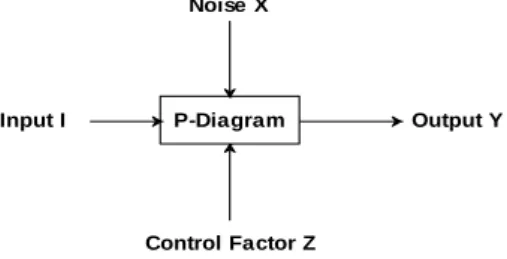
Figure 1. P-diagram for any problem. Here “P” stands for process

Figure 1 shows the P-diagram where noise (Noise X) is present in the process. The primary objective of Taguchi approach is to achieve the optimized output (Output Y), noise should have no effect and therefore to reduce the variations in the output even though the noise is present and hence the process can be called as robust. Control factor Z is shown to be present and need special attention for the optimization problems since optimization problem involves finding the suitable control factor levels so that the best output is at the target value. Orthogonal arrays is found effective in setting the balanced experiments and Taguchi signal-to-noise ratios (SNR), which are log functions of the desired output serve as an objective functions for optimization helps in data analysis and prediction of optimum results [27].

3.3.3 Response surface design

It helps in examine the relationship between a response and a set of factors or experimental variables. This method is mainly employed after indentifying a “vital few” controllable experimental variables and the author is interested in finding appropriate setting that optimizes the response. The main objective of applying design of this type is to develop a model that describes a continuous curve, or surface, that connects the measured data at strategically important places in the experimental window. Response surface design takes the merits of a least-squares curve fit or regression analysis to identify the appropriate model tests, the validity of the model and finally analyze the model.

4. CASE STUDY: GRAMMAR INDUCTION SYSTEM

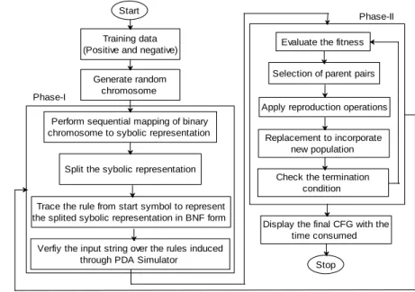
It is evident that GAs are being applied for search and optimization problems where the search space is large, complex and contains possible difficulties, like high dimensionality, multimodality, discontinuity and noise. GA uses biology inspired and survival of the fittest mechanism to refine a set of solution in an iterative manner [11] [17]. It works on encoding mechanism to represent a population of solution. Fitness is the measure of GA and an individual‟s fitness is directly related to the objective/fitness function for an optimization problem. Using various reproduction operators the individual population can be modified to a new population [1]. The search process terminates when reaches to termination condition or to the threshold. In this section, the author has presented a block diagram, shows the process of the GI uses GA as shown in Figure 2. The overall process has been divided into two different phase. The Phase-1 is responsible for production rule generation and verification, whereas Phase-2 shows the steps of GA incorporated to optimize the search process and explore the search space adequately.

The GI process starts generating the initial random binary chromosome (BC), which is then mapped to appropriate symbolic chromosome (SC) representation of terminals and non-terminals in a sequential manner. The SC has been divided into equal block size of five equal to production rule length. Each SC has been traced from the start symbol „S‟ to terminal to remove use less production and rest of the productions have been tested for removal of left recursion, unit production, ambiguity and left factor. A string to be tested has been selected and passed for the validity, i.e. acceptability of the CFG equivalent to the chromosome. The test string and the CFG rules are the input to the finite state controller, which verifies the acceptability through the proliferation on the pushdown automata (PDA).

P-Diagram Output Y

Noise X

Control Factor Z Input I

Figure 2. Block diagram for context free grammar induction using GA.

A random initial binary chromosomes (BC) consist of sequence of 0‟s and 1‟s have been created in Figure 4. The BC is mapped into terminals and non-terminals in a sequential manner following 3-bit/4-bit coding that depend on the number of symbols present in the language. If more than two symbols are used in the language then 4-bit representation has been used otherwise use 3-bit representation. The start symbol „S‟ has been mapped at “000” and „?‟ represents the null symbol mapped at “010”, whereas for others symbols (terminals and non-terminals) are used as appropriate.

Binary chromosome:

000100010000010010000101001111000101000110010000010011101011001000011001001110101010001 100000100010110110000001101101110

Coding of terminal and non-terminals

Non-terminals Terminals

S  000 1100

A001 0101

B111 ?010

C011 ?110

Symbolic chromosome representation: S1?S??S0ABS0S??S?C0CASCAA?0?A1S1???SA00?

The SC‟s are divided into block size of five equal to the production rule length as shown in Table 2, which are then traced from „S‟ to remove the insufficiency presents. The PDA simulator accepts test string and the production rules as an input for any specific language, verifies the acceptability via proliferation on the PDA.

The fitness of an individual has been calculated in each GA run and then selection of parent string is done. In GI problem, the fitness of an individual chromosome largely depends upon the acceptance (rejection) of the positive and negative sample strings. The fitness value increase for accepting positive (AP) and rejecting negative (RN) sample, whereas it decreases for accepting negative (AN) and rejecting positive (RP) sample. The problem specific factor (s) also plays a significant role in GA‟s performance. In case of GI, production rule length (PR) is an important factor, has been considered in the fitness calculation. Equation (2) has been applied to calculate the fitness of an individual.

*((

) (

)) (2*

)

Fitness





C

AP RN





AN



RP



C



PR

Training data (Positive and negative)

Generate random chromosome

Perform sequential mapping of binary chromosome to sybolic representation

Split the sybolic representation

Trace the rule from start symbol to represent the splited sybolic representation in BNF form

Verfiy the input string over the rules induced through PDA Simulator

Evaluate the fitness

Selection of parent pairs

Apply reproduction operations

Replacement to incorporate new population Check the termination

condition

Display the final CFG with the time consumed Phase-I

Phase-II Start

The following convention has been followed for the selection of the best grammar rules: “A grammar that accepts all the positive strings and rejects the entire negative string from set of training data with minimum number of production rules”. The value of constant (C= 10) is found sufficient to accommodate grammar rules blocks present in the symbolic chromosome.

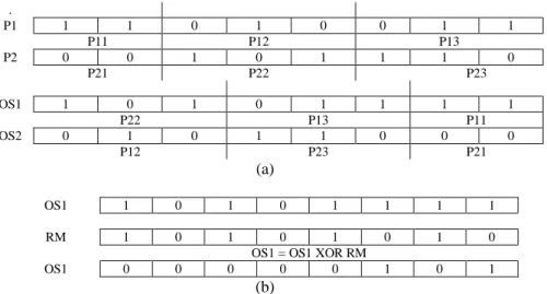
The GA‟s performance largely depends on the two most commonly used genetic operators are crossover and mutation. The operators‟ crossover and mutation play a significant role in the population diversity management and therefore improves the convergence speed. A variation of two point crossover based on the cyclic crossover has been incorporated to perform the crossover operation. The inverted mutation method has been applied with random mask. As we know the mutation operator introduces diversity in the population helps to keep the search process alive. Random mask is useful in achieving the diversity. The following convention has been applied: “simply apply “XOR” operation between the parent strings received after crossover operation and the random offspring”. An example for both crossover and mutation operations have been represented in Figure 3.

.

P1 1 1 0 1 0 0 1 1

P11 P12 P13

P2 0 0 1 0 1 1 1 0

P21 P22 P23

OS1 1 0 1 0 1 1 1 1

P22 P13 P11

OS2 0 1 0 1 1 0 0 0

P12 P23 P21

(a)

OS1 1 0 1 0 1 1 1 1 RM 1 0 1 0 1 0 1 0

OS1 = OS1 XOR RM

OS1 0 0 0 0 0 1 0 1 (b)

Figure 3. Demonstrations of crossover and mutation operations. (a) Representing the two point cut crossover based on cyclic crossover. (b) Inverted mutation by generating random mask (RM) and then applying XOR

operation.

5. RESULTS AND ANALYSIS

Experiments have been conducted on the set of regular as well as context free languages. The set of positive and negative corpora have been chosen with varying patterns of 0‟s and 1‟s is given in Table 1.

Table 1. Test Languages Description L-id Descriptions Standard Set

L1 (10)* over (0 + 1)* Tomita [30] / Dupont [9] L2 All string not containing „000‟ over (0+1)* ---

L3 Balanced Parentheses Huijsen [18]/ Keller and Lutz [19] L4 Odd binary number ending with 1 Dupont [9]

L5 Even binary number ending with 0 over (0+1)* Dupont [9]

The implemented GA utilizes two points cut crossover based on the cyclic crossover and inverted mutation with random mask for CFG induction. Java programming on Net Beans IDE 7.0.1, Intel CoreTM 2processor (2.8 GHz) with 2 GB RAM are used.

Table 2 shows the parameters used in implementation of the proposed algorithm. Minimum description length principle (MDLP) has been used to generate the positive and a negative string set required during the execution [15] [19]. For selecting the corpus, strings of terminals are generated for the length

L

from the given language. Initially, L= 0 is chosen, which gradually increases up to the required length to represent the language features. The valid and the invalid strings generated will be considered as positive and negative strings respectively.

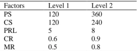
Table 2. Selected factors and their levels Factors Level 1 Level 2 PS 120 360 CS 120 240 PRL 5 8 CR 0.6 0.9 MR 0.5 0.8

The performance of GA largely depends on PS, CS, CR, and MR. and in GI production rule length is considered as an important factor that affects the results. In the present scenario, orthogonal array involves five control factors with two levels have been used shown in Table 2. Both full factorial and Taguchi approach have been applied for the estimation purpose. The aim of applying both the approaches is not only to identify the suitable parameters value but also to discuss the suitability of these approaches on the realistic problems.

5.1. Taguchi Design for Parameter Quantification

Table 3 presents Taguchi design, each row of the design specifies a combination of factor level, used for a run of the experiment. Taguchi approach utilizes orthogonal arrays referred as Taguchi orthogonal arrays, which require only a fraction of the full factorial combinations. The primary goal is to find factor setting. Table 3 tells the number of runs/ experiment numbers, factors and levels for each factor in the design. In the present scenario, orthogonal array design consists of 5 factors, 2 levels and 8 runs, which can be represented as L8 (2**5). To analyze the Taguchi design one need to understand the effect of control and noise factors on the response, then select the best combination of factor setting for conducting the experiment/process. Equation (3) is used to evaluate signal-to-noise ratio.

2

1

10log

u

N u i

u i

y

SNR

N





 

_

_







Where,

i

u

N

y

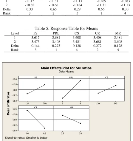
Table 4 and Table 5 show the response table for signal to noise ratios and means respectively. The results of twenty runs over randomly chosen language sets as shown in Table 1, is considered as trial. Delta and rank measure the size of the effect by taking the difference whereas rank explains the order of the control factor based on the value of delta. It can be seen from Table 4 that CR (rank: 1, since delta: 0.66) has the largest effect on the results yields, whereas CS (rank: 5, delta: 0.29) has the smallest effect. Similarly, Table 5 shows the response table for means.

The response in Table 4 for signal to noise ratios indicates that smaller is better, therefore combination PS: 120, PRL: 5, CS: 120, CR: 0.9 and MR: 0.8 shown in Table 3 experiment number 2 is taken for the robust process design and conduct the experiments since this combination produces smaller SNR i.e. -12.1889. The effects of these factors are shown in Figure 4 indicates that the each factor line is not horizontal; hence there is main effect present. Also, it can be seen that different levels of the factor affect the characteristic in different manner. The greater the difference in the vertical position indicates the greater the magnitude in the main effect and the comparison in the slope lines explains the relative magnitude of the factor effects. For the grammar inference problem, the main effect of the signal to noise ratio is depicted in Figure 4 indicates that CR has the greatest effect on the SNR. The experiment with CR 0.9 shows much smaller SNR than the experiment with CR 0.6. Response table helps in selection of the best level factor using delta and rank values shows greatest effect on each response characteristic. In some situation, the best level of a factor for one response may differ from the best level for another response characteristic. To resolve the situation like this, predict the results for several other combinations of factors levels to find the appropriate combination produces the best outcome.

Linear model analysis for SNR versus the parameters (PS, PRL, CS, CR and MR) is shown in Table 6. Coefficients for each factor levels are calculated. The regression coefficient can be utilized to determine which of our factors are statistically significant with the help of p-value, given in the last column of Table 6. If p-value is less than or equal to α-level (0.05), then conclude that the effect is significant otherwise the effect is not significant.

Table 3. Parameter selection by orthogonal array method

Ex.No. PS PRL CS CR MR Means Coff. Variation Std.dev. SNR 1 120 5 120 0.6 0.5 3.56667 0.0428278 0.152753 -11.0506 2 120 5 120 0.9 0.8 4.06667 0.0375621 0.152753 -12.1889 3 120 8 240 0.6 0.5 3.26667 0.0467610 0.152753 -10.2884 4 120 8 240 0.9 0.8 3.56667 0.0901276 0.321455 -11.0687 5 360 5 240 0.6 0.8 3.50000 0.0285714 0.100000 -10.8837 6 360 5 240 0.9 0.5 3.59000 0.0460243 0.165227 -11.1080 7 360 8 120 0.6 0.8 3.30000 0.0606061 0.200000 -10.3809 8 360 8 120 0.9 0.5 3.50000 0.0494872 0.173205 -10.8884 SNR: Signal to noise ratio

Table 4. Response Table for Signal to Noise Ratios (Smaller is better) Level PS PRL CS CR MR

1 -11.15 -11.31 -11.13 -10.65 -10.83 2 -10.82 -10.66 -10.84 -11.31 -11.13 Delta 0.33 0.65 0.29 0.66 0.30

Rank 3 2 5 1 4

Table 5. Response Table for Means

Level PS PRL CS CR MR 1 3.617 3.681 3.608 3.408 3.481 2 3.473 3.408 3.481 3.681 3.608 Delta 0.144 0.273 0.128 0.272 0.128 Rank 3 1 4 2 5

360 120

-10.6 -10.8 -11.0 -11.2 -11.4

8

5 120 240

0.9 0.6

-10.6 -10.8 -11.0 -11.2 -11.4

0.8 0.5

PS

M

ea

n

of

S

N

ra

ti

os

PRL CS

CR MR

Main Effects Plot for SN ratios

Data Means

Signal-to-noise: Smaller is better

Figure 4. Main effects plot for signal to noise (smaller is better)

Table 6. Linear Model Analysis: SN ratios versus PS, PRL, CS, CR, MR (Estimated Model Coefficients for SN ratios)

Term Coef. SE Coef. T P Constant -10.9822 0.05706 -192.453 0.000

PS -0.1669 0.05706 -2.925 0.100 PRL -0.3256 0.05706 -5.706 0.029 CS -0.1450 0.05706 -2.541 0.126 CR 0.3313 0.05706 5.806 0.028 MR 0.1483 0.05706 2.600 0.122 S= 0.1614 R-Sq= 97.8% R-Sq (adj)= 92.2%

Table 7. Linear Model Analysis: SN ratios versus PS, PRL, CS, CR, MR (Analysis of Variance for SN ratios) Source DF Seq SS Adj SS Adj MS F P

PS 1 0.22293 0.22293 0.22293 8.56 0.100 PRL 1 0.84804 0.84804 0.84804 32.55 0.029 CS 1 0.16817 0.16817 0.16817 6.46 0.126 CR 1 0.87809 0.87809 0.87809 33.71 0.028 MR 1 0.17604 0.17604 0.17604 6.76 0.122 Residual Error 2 0.05210 0.05210 0.02605

Total 7 2.34538

Table 8. Linear Model Analysis: Means versus PS, PRL, CS, CR, MR (Estimated Model Coefficients for Means)

Term Coef. SE Coef. T P Constant 3.54458 0.02853 124.233 0.000

PS 0.07208 0.02853 2.526 0.127 PRL 0.13625 0.02853 4.775 0.041 CS 0.06375 0.02853 2.234 0.155 CR -0.13625 0.02853 -4.775 0.041 MR -0.06375 0.02853 -2.234 0.155 S= 0.08070 R-Sq= 96.9% R-Sq (adj)= 89.1%

Table 9. Linear Model Analysis: Means versus PS, PRL, CS, CR, MR (Analysis of Variance for Means) Source DF Seq SS Adj SS Adj MS F P

PS 1 0.04157 0.04157 0.041568 6.38 0.127 PRL 1 0.14851 0.14851 0.148513 22.80 0.041 CS 1 0.03251 0.03251 0.032513 4.99 0.155 CR 1 0.14851 0.14851 0.148513 22.80 0.041 MR 1 0.03251 0.03251 0.032513 4.99 0.155 Residual Error 2 0.01303 0.01303 0.006513

Total 7 0.41664

Figure 5. Residual plot for signal to noise ratios

Having seen the obtained p-value in Table 6, one can conclude that the p-value of PRL and CR is less than the α-level, i.e. for PRL (0.029 < 0.05) and for CR (0.028 < 0.05), hence we can conclude that the effect of PRL and CR are statistically significant, whereas for other factor‟s obtained p-value is higher than the α-level (0.05), therefore the effect is not significant for PS, CS and MR or they are significantly related to the response.

Analysis of variance for SN ratio is given in Table 7, used to analyze the linear model based on the p-value. To evaluate the effect of an individual factor, one needs to identify the p-value. The p-value of PRL and CR is less than the α-level; conclude that the effect is significant, while the remaining factors are significantly related to the response.

Table 8 and Table 9 presents the linear model analysis using coefficient for means and analysis of means for the chosen factors. Having seen these tables one can conclude that factors PRL and CR has

0.2 0.1 0.0 -0.1 -0.2 99 90 50 10 1 Residual P e rc en t -10.0 -10.5 -11.0 -11.5 -12.0 0.10 0.05 0.00 -0.05 -0.10 Fitted Value R e si d u a l 0.10 0.05 0.00 -0.05 -0.10 2.0 1.5 1.0 0.5 0.0 Residual F re q u e n cy 8 7 6 5 4 3 2 1 0.10 0.05 0.00 -0.05 -0.10 Observation Order R e si du a l

Normal Probability Plot Versus Fits

Histogram Versus Order

significant effect on the response, since the obtained p-value for both the factor is less than the p-value, whereas the remaining factors showing the significant related response.

The residual plots for SNR are depicted in Figure 5, presents four residual plot in one window. Residual plot is a useful to determine whether the model meets the assumptions of the analysis. Figure 5 includes four graphs such as: normal probability plot, histogram, residual versus fitted value, and residual versus order of the data. Normal probability plot can be utilized to see whether the data are normally distributed or not. It also indicates whether other variables are influencing the response, or outlier exists in the data or not. Normal probability plot shown in Figure 5 do not appear to follow a straight line but it is also uncertain whether or not there is evidence or non-normality, skewness, outliers since there are few observations collected. Histogram of the residual presents the distribution of the residuals for all the observations. Histogram can be utilized as an exploratory tool to understand the characteristics of the data depending on the spread or variation and shape of the histogram. Residual histogram should be bell shaped, which can be used to test the skewness and outlier. It can be seen, histogram depicts a bell shaped curve between the interval (-0.05 and + 0.05), therefore one can say that the data is normally distributed. Residual versus fitted value plot test whether residual is scattered randomly about zero. Using this plot one can see uneven spreading of residual across the fitted values, which indicates non-constant variance. It can also be utilized to assess nature of plot for curvilinear and outlier. Based on the plot shown in Figure 5 the residuals appear to be randomly scattered about zero. Also, plot does not show any evidence of non-constant variance and outlier and missing terms. Residual versus order of the data plot is also presented in Figure 5. It is given to plot the residuals in the order of the corresponding observations. This plays an important role when the order of the observations may influence the response. In addition, the features of this plot can be utilized particularly in a designed experiment in which the runs are not randomized. To examine the plot, check, if any correlation exists between error terms that are near to each other. Correlation can be signified by an ascending/descending trend in the residuals and rapid change in signs of adjacent residuals. Having seen the plot, the residuals are randomly scattered about zero since there is ascending/descending trends in the residuals. Also it shows rapid change in signs of adjacent residuals.

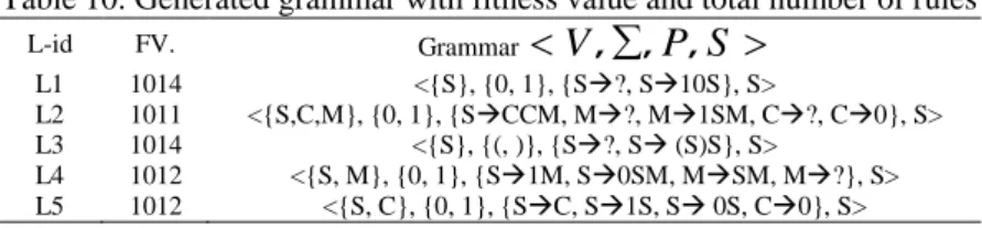
Table 10. Generated grammar with fitness value and total number of rules L-id FV. Grammar



V

, , ,



P S



L1 1014 <{S}, {0, 1}, {S?, S10S}, S>

L2 1011 <{S,C,M}, {0, 1}, {SCCM, M?, M1SM, C?, C0}, S> L3 1014 <{S}, {(, )}, {S?, S (S)S}, S>

L4 1012 <{S, M}, {0, 1}, {S1M, S0SM, MSM, M?}, S> L5 1012 <{S, C}, {0, 1}, {SC, S1S, S 0S, C0}, S>

The GA is a stochastic search technique and therefore, the results are collected as the average of twenty runs for each language. The GA search process continues until it reaches to a maximum number of generations or reaches to threshold, where threshold indicates the highest rank solution‟s fitness. The results show that the presented approach is capable for CFG induction. Minimum description length (MDL) principle is applied to generate a proportionate number of positive and negative sample strings. The crossover and mutation methods have been found effective in improving the performance and exploring the search space. It was observed that the MDL principle works effectively in selecting the correct sample strings with minimum description length. For the validation purpose experimentally obtained grammars have been tested against the best known available grammar. The standard representation



V

, , ,



P S



Table 11 presents threshold value, i.e. total number of generations required to produce the best solution, the time consumed in milliseconds, generation range, mean and standard deviation. Results are collected as the average of successful twenty runs. The number of generations taken over twenty generation run varies, therefore generation range is given. The phenomenon involved with generation range can be understood with the help of an example: the generation range for L1 is 4±2, means the number of generations taken over twenty generation run varies between 02 (4 – 2) and 06 (4 + 2) similarly for others. During the computational experiment, the author found that the GA produced better results in terms of convergence time and showed less tendency of premature convergence. Incorporating the experimental design approach helps in identifying the appropriate parameters value that makes the system robust and improves the overall performance.

Figure 6. Best average fitness with respect to generations chart for each language L1 through L5

Table 11. Threshold, time consumed generation range, mean and standard deviation for each language. L-id Threshold Time Generation Range Mean Std. Dev.

L1 9 68671.3 4±2 3 2.75 L2 30 4693783 12±9 17.5 6.64 L3 10 205309.5 4±3 6.7 2.26 L4 12 305396.7 7±3 6.9 3.31 L5 13 366416.1 9±5 8.8 2.97

6. CONCLUSION

In this paper, a GA has been presented for CFG induction from positive and negative samples. The GA has the merit of powerful global exploration capabilities, which can exploit the optimum offspring. To achieve the robust experiment design two most popular approaches have been discussed and demonstrated over CFG induction problem. Various factors affect the overall working of the GA. The author has taken five factors with 2-level in consideration in tuning process. Taguchi approach has been incorporated for the GA‟s parameters quantification and found working successfully. It was observed that Taguchi design require one fourth of the full factorial design in finding the right combination of the parameters and consumes less time because it runs the experiments less time than full factorial design. It is demonstrated that for five control factors with 2-level eight combinations were used in case of Taguchi design. The GA presented in this paper utilizes two point cyclic based crossover and inverted mutation with random offspring; these operators were found effective in maintaining diversity in the population and direct the GA‟s search towards the global optimum. The author has executed the GA for context free and regular languages of varying complexities. The experimental results have been found encouraging because the GA implemented is found capable in CFG induction and greatly improves the performance, showed less tendency of local optimum convergence.

The result reported in this paper provide a way of design a robust experiments design can be utilized for the performance enhancement of the GA in terms of computational time, quality of results and one of the mechanism in addressing premature convergence. This paper discusses a number of features key aspects one need to understand in constructing a robust GA. The author believe that the observations and results reported will be helpful for the researchers in develop good experiment design because if someone want to develop a GA for solving an optimization problem, then these observations and discussion will direct them in selecting the right factors correctly for robust designing. This paper has shown some aspects of a GA, which are really important to study and more such studies are required to understand better working principle of GA. An obvious outcome of this study would be development of an improved GAs.

REFERENCES

[1] Amor, H. B., and Rettinger, A. Intelligent exploration for genetic algorithms: Using self-organizing maps in

evolutionary computation. In Proceedings of the 7th annual conference on Genetic and evolutionary computation

(pp. 1531-1538). ACM, 2005

[2] Angluin, D. Inductive inference of formal languages from positive data. Information and control, 45(2), 117-135,

1980.

[3] Angluin, D., and Smith, C. H. Inductive inference: Theory and methods. ACM Computing Surveys (CSUR), 15(3),

237-269, 1983.

[4] Angluin, D. Queries and concept learning. Machine learning, 2(4), 319-342, 1988.

[5] Albus, J. E., Anderson, R. H., Brayer, J. M., DeMori, R., Feng, H. Y., Horowitz, S. L. and Vamos, T.. Syntactic

[6] Bagchi, T. P., and Deb, K. Calibration of GA parameters: the design of experiments approach. Computer Science and Informatics, 26, 46-56, 1996.

[7] Choubey, N. S., Kharat, M. U., and Pandey, H. M. Developing Genetic Algorithm Library Using Java for CFG

Induction. International Journal of Advancement in Technology, 2011.

[8] Delgado, M., and Pegalajar, M. C. A multiobjective genetic algorithm for obtaining the optimal size of a recurrent

neural network for grammatical inference. Pattern Recognition, 38(9), 1444-1456, 2005.

[9] Dupont, P. Regular grammatical inference from positive and negative samples by genetic search: the GIG method.

In Grammatical Inference and Applications (pp. 236-245). Springer Berlin Heidelberg, 1994.

[10] Fowlkes, W. Y., and Creveling, C. M. Engineering methods for robust product design. Addison-Wesley, 1995.

[11] Golberg, D. E. Genetic algorithms in search, optimization, and machine learning. Addion Wesley, 1989.

[12] Gold, E. M. Language identification in the limit. Information and control, 10(5), 447-474, 1967.

[13] Gupta, M. C., Gupta, Y. P., and Kumar, A. Minimizing flow time variance in a single machine system using

genetic algorithms. European Journal of Operational Research, 70(3), 289-303, 1993.

[14] Harrison, M. A. Introduction to formal language theory. Addison-Wesley Longman Publishing Co., Inc., 1978.

[15] Hansen, M. H., and Yu, B. Model selection and the principle of minimum description length. Journal of the

American Statistical Association, 96(454), 746-774, 2001.

[16] Hsieh, C., Chou, J., and Wu, Y. Taguchi-MHGA method for optimizing grey-fuzzy gain-scheduler. In Proceedings

of the 6th International Conference on Automation Technology, Taiwan (pp. 575-582), 2000.

[17] Holland. Adaptation in natural and artificial systems: an introductory analysis with applications to biology, control,

and artificial intelligence. MIT press, 1992.

[18] Huijsen, W. O. Genetic grammatical inference. In CLIN IV. Papers from the Fourth CLIN Meeting, Vakgroep

Alfa–informatica (pp. 59-72), 1993.

[19] Keller, B., and Lutz, R. Evolving stochastic context-free grammars from examples using a minimum description

length principle. In 1997 Workshop on Automata Induction Grammatical Inference and Language Acquisition,

1997.

[20] Klint, P., Lämmel, R., and Verhoef, C. Toward an engineering discipline for grammarware. ACM Transactions on

Software Engineering and Methodology (TOSEM), 14(3), 331-380, 2005.

[21] Lang, K. J. (1992). Random DFA's can be approximately learned from sparse uniform examples. In Proceedings of

the fifth annual workshop on Computational learning theory (pp. 45-52). ACM, 1992.

[22] Oliveira, A. L. (Ed.). Grammatical Inference: Algorithms and Applications: 5th International Colloquium, ICGI

2000, Lisbon, Portugal, September 11-13, 2000 Proceedings. Springer, 2004.

[23] Pakath, R., and Zaveri, J. S. Specifying critical inputs in a genetic driven decision support system: An automated

facility. Department of Decision Science and Information Systems, College of Business and Economics, University

of Kentucky, Lexington, 1993.

[24] Pandey, H. M., Chaudhary, A., and Mehrotra, D. A comparative review of approaches to prevent premature

convergence in GA. Applied Soft Computing, 24, 1047-1077, 2014.

[25] Pandey, H. M., Dixit, A., and Mehrotra, D. Genetic algorithms: concepts, issues and a case study of grammar

induction. In Proceedings of the CUBE International Information Technology Conference (pp. 263-271). ACM,

2012.

[26] Pandey, H. M. Context free grammar induction library using Genetic Algorithms. In Computer and Communication

Technology (ICCCT), 2010 International Conference on (pp. 752-758). IEEE, 2010.

[27] Roy, R. K. Design of experiments using the Taguchi approach: 16 steps to product and process improvement. John

Wiley & Sons, 2001.

[28] Schaffer, J. D., Caruana, R. A., Eshelman, L. J., and Das, R. A study of control parameters affecting online

performance of genetic algorithms for function optimization. In Proceedings of the third international conference

on Genetic algorithms (pp. 51-60). Morgan Kaufmann Publishers Inc., 1989.

[29] Stevenson, A., and Cordy, J. R. Grammatical inference in software engineering: an overview of the state of the art.

In Software Language Engineering (pp. 204-223). Springer Berlin Heidelberg, 2013.

[30] Tomita, M. Dynamic construction of finite-state automata from examples using hill-climbing. In Proceedings of the

fourth annual cognitive science conference (pp. 105-108), 1982.

[31] Unal, R., and Dean, E. B. Taguchi approach to design optimization for quality and cost: an overview. In Annual

conference of the international society of parametric analysts (Vol. 1), 1991.

[32] Valiant, L. G. A theory of the learnable. Communications of the ACM, 27(11), 1134-1142, 1984.

[33] Yang, W. P., and Tarng, Y. S. Design optimization of cutting parameters for turning operations based on the

Taguchi method. Journal of materials processing technology, 84(1), 122-129, 1998.

BIOGRAPHY OF AUTHOR

Hari Mohan Pandey did M.Tech in Computer Engineering from Mukesh Patel School of Technology Management & Engineering, NMIMS University, Mumbai. He is perusing Ph.D. in Computer Science & Engineering. He has published research papers in various journals. He has written many books in the field of Computer Science & Engineering for McGraw-Hill, Pearson Education, and University Science Press. He is associated with various International Journals as reviewer and editorial board member. His area of interest Machine Learning Computer, Artificial Intelligence, Soft Computing etc.