Preprint typeset using LATEX style AASTeX6 v. 1.0
A SEARCH FOR RAPIDLY PULSATING HOT SUBDWARF STARS IN THE GALEX SURVEY
Thomas M. Boudreaux1, Brad N. Barlow1, Scott W. Fleming2, Alan Vasquez Soto1, Chase Million3, Dan E.
Reichart4, Josh B. Haislip4, Tyler R. Linder5, and Justin P. Moore4
1Department of Physics, High Point University, One University Parkway, High Point, NC 27268, USA
2Space Telescope Science Institute, 3700 San Martin Dr. Baltimore, MD 21218, USA
3Million Concepts LLC, PO Box 119, 141 Mary St, Lemont, PA 16851, USA
4Department of Physics and Astronomy, University of North Carolina, Chapel Hill, NC 27599, USA
5Department of Physics, Eastern Illinois University, 600 Lincoln Ave., Charleston, IL 61920, USA
(Received June 1, 2017; Revised June 28, 2017; Accepted June 28, 2017)
ABSTRACT
NASA’s Galaxy Evolution Explorer (GALEX) provided near- and far-UV observations for approxi-mately 77 percent of the sky over a ten–year period; however, the data reduction pipeline initially only released single NUV and FUV images to the community. The recently released Python mod-ule gPhoton changes this, allowing calibrated time–series aperture photometry to be extracted easily from the raw GALEX data set. Here we use gPhoton to generate light curves for all hot subdwarf B (sdB) stars that were observed by GALEX, with the intention of identifying short–period, p-mode pulsations. We find that the spacecraft’s short visit durations, uneven gaps between visits, and dither pattern make the detection of hot subdwarf pulsations difficult. Nonetheless, we detect UV variations in four previously known pulsating targets and report their UV pulsation amplitudes and frequencies. Additionally, we find that several other sdB targets not previously known to vary show promising signals in their periodograms. Using optical follow–up photometry with the Skynet Robotic Telescope Network, we confirmp-mode pulsations in one of these targets, LAMOST J082517.99+113106.3, and report it as the most recent addition to the sdBVr class of variable stars.
Keywords: stars: oscillations
1. INTRODUCTION
Hot subdwarf B stars (sdBs) are extreme horizontal branch stars believed to have formed from red giants that lost their outer H envelopes while ascending the red giant branch, likely due to interactions with a nearby companion (Heber 2016). The leftover core of the pro-genitor star — which becomes an sdB upon core He ignition —has an effective temperature 22000≤Teff ≤ 40000 and a surface gravity 5.0 ≤logg ≤6.2. Theory predicts sdBs should have masses around 0.5 M, which
is generally consistent with reported observations (Han
et al. 2003).
Subdwarf B stars are quite common, outnumbering white dwarfs down to magnitude B∼18; despite this, they are one of the less well understood branches of stel-lar evolution. sdBs play interesting roles in our under-standing of several astrophysical phenomena, including the effects of main sequence evolution interrupted by binary interactions, the UV–upturn in giant elliptical galaxies (Brown et al. 1997), the “second-parameter” problem in globular cluster morphology (e.g., Moni
Bidin et al. 2008), and even sub-luminous Type 1a
su-pernovae (e.g., Geier et al. 2013). Luckily, some hot
subdwarfs pulsate, and these pulsations serve as efficient probes of the interior structures and dynamics that drive this phase of stellar evolution.
The first pulsating sdB (sdBV) star, EC 14026-2647, was discoverd two decades ago byKilkenny et al.(1997); since then, over 100 such pulsators have been uncov-ered. sdBV stars come in three main flavors: (i) the sdBVr stars, which exhibit rapid, acoustic–mode (p– mode) oscillations with periods from 1-10 minutes and amplitudes typically<20 parts per thousand (ppt); (ii) the sdBVs stars, which exhibit slow, gravity–mode (g– mode) oscillations with periods from 1–2 hours and am-plitudes around a few ppt; and (iii) the hybrid sdBVrs stars, which exhibit both p–mode and g–mode oscilla-tions. Past asteroseismological studies of sdB stars, es-pecially those using data from theKeplermission, have led to precise measurements of sdB masses, radii, rota-tion rates, and other parameters (e.g., Østensen et al. 2014). The first step to unlocking the potential of aster-oseismology is, of course, the discovery of new pulsating stars. Most studies of sdBV stars and searches for new pulsators have taken place in optical bandpasses, even though the sdB Planck distribution peaks in the UV and
most sdBV pulsation modes have higher amplitudes in the UV compared to the optical (Heber 2016).
NASA’s Galaxy Evolution Explorer (GALEX, Martin
et al. 2005) provides a unique opportunity to study
vari-able hot subdwarf stars, due to its large field coverage in UV bands. Launched in 2003, GALEX observed 77% of the sky through two broadband UV filters, centered around 1728 ˚A (“FUV”) and 2271 ˚A (“NUV”). The original data reduction pipeline yielded calibrated im-ages of each field at a full visit depth. These, along with source catalogs, compose the primary, mission-produced archive products (Morrissey et al. 2007). However, due to GALEX’s use of micro–channel plate detectors (MCP), which recorded the individual photon events with a high degree of time accuracy, the raw GALEX data set does contain time series information. A Mikul-ski Archive for Space Telescopes (MAST) archive soft-ware tool called gPhoton extracts calibrated time series information on demand from the raw data by substan-tially reproducing key functionality from the GALEX mission calibration pipeline (Million et al. 2016).
Here we present a search for short–period sdB pulsa-tions in the archived GALEX dataset using gPhoton. An initial sample of 5613 hot subdwarfs (Geier et al. 2016), which represents a good approximation of all cat-aloged hot subdwarf stars, was down-selected based on magnitudes, coordinates and total exposure time avail-able in the gPhoton database, described fully in Section
2. These selection criteria yielded 1881 targets upon which we focused our investigation. Calibrated light curves with time bins of 30 seconds were generated for each target using gPhoton. We identify NUV pulsations consistent with previous optical observations for four known pulsating sdB stars. Additionally, we identify several new candidate pulsators that show signals con-sistent with those of pulsating sdBs, and confirm one of these as a new sdBVrstar with ground–based follow–up observations.
2. DATA REDUCTION WITH GPHOTON
We used the gPhoton software package to produce cal-ibrated light curves of all sdB targets. To generate light curves, the gPhoton tool called gAperture integrates sky-mapped GALEX photon events, produced by the mission with time resolutions of five microseconds, over user-defined time bins and photometric apertures, ap-propriately calibrated for detector exposure time and relative response (Million et al. 2016). The gPhoton package also includes a tool called gFind for quickly de-termining available exposure time coverage of specific targets and a tool called gMap for generating image and “movie” files of GALEX observations. We made use of gFind, gMap and gAperture to select targets, create 2D and 3D FITS images, and generate photometrically
cal-ibrated light curves, respectively.
For each target, we extracted target ID, source posi-tion (as right ascension and declinaposi-tion in J2000 decimal degrees), V magnitude, and GALEX NUV magnitude when available. Note that due to both higher flux val-ues and wider GALEX coverage in the NUV compared to the FUV, we focused our efforts on NUV measure-ments. Targets that fall outside of our acceptable mag-nitude range (13≤N U V ≤19) are rejected. This cut conservatively eliminates bright sources that will trig-ger non–linear detector response and dim sources with poor signal–to–noise. All remaining targets then have their coordinates queried using gFind, which returns a data structure containing the total available expo-sure time, the nearest GALEX merged catalog (MCAT) source, and a breakdown of visits. Note that the MCAT is the mission-produced catalog of detected sources for all GALEX visits, but does not account for duplicate sources due to field overlaps. Also note that a “visit” is the amount of time spent by GALEX observing a given pointing while the spacecraft was behind earth’s shadow, and can be no longer than 30 minutes in duration.
GALEX conducted three main surveys: the All-sky Imaging Survey (AIS), Medium-imaging Survey (MIS), and Deep-imaging Survey (DIS). The All-sky Imaging Survey took∼100s integrations (Morrissey et al. 2007), too short to be useful for our investigation. Conse-quently we only investigate data from MIS (∼1500s) and DIS (∼30000s). We use the key ‘expt’ in both NUV and FUV to select only those targets that have more than 600s in either band; this 600s cut is also used as the filter for AIS observations . After the ini-tial 5613 sdBs provided byGeier et al.(2016) were run through these criteria, we find 1881 targets with a suf-ficient amount of GALEX observation time to allow for pulsation searches. These targets were each visited by the spacecraft between 1 and 375 times, with a mean (median) of 7.4 (4) visits per target. The visit lengths ranged from 10–30 min, with an average visit length of about 15.5 min.
We used gMap to produce both full depth (coadd) im-ages of targets using all available GALEX observations and movie files of targets with ten second integrations / frames across all available observations. A custom Python tool (FaRVaE1) was developed to automatically define the radius of the photometric aperture and the radii of the inner and outer annuli used to determine the background. The tool makes use of SEP, a software suite used to conduct aperture photometry based on Source Extractor (Barbary 2016;Bertin & Arnouts 1996). Each
FITS image and cube were read into FaRVaE, where the auto-definition routine was run. We then manually veri-fied the quality of these parameters by eye. Specifically, we ensure that there are as few bright sources in the annulus as possible, and that all visible flux is included in the aperture. We also took the opportunity to visu-ally check the images for any obvious contamination of the detector hotspot mask into the target or for obvious astrophysical flaring activity.
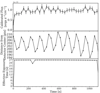
The aperture and annulus definition files were used as inputs to the gAperture module to generate aper-ture photometry at 30-second bins. We settled on this particular exposure time since longer cycle times would have associated Nyquist frequencies below those of some known sdB pulsations, and shorter exposure times would decrease the signal-to-noise ratio in each bin to levels that would make pulsation detection difficult, especially for low amplitudes. Due to the computationally expen-sive nature of a gAperture call, a consequence of net-work bandwidth and available computational resources, we ran the majority of gAperture calls on a cluster local to the MAST in Baltimore. Each target was run as a separate job on a 64-core machine to allow for multiple targets to run through gAperture at a time. All tar-gets run through gAperture and gMap produced a total of 20 GBs of data, including images and light curves. Extracted output includes raw counts, calibrated fluxes, effective exposure time of each bin after accounting for dead time, the mean observation time of each bin, the mean position of the target on the detector during each bin, and associated errors. Consult the gPhoton User’s Guide for a detailed description of all the available out-put2. An example of gPhoton output for one of our targets is shown in Figure1.
3. DATA ANALYSIS
Given the large number of light curves generated by gPhoton (13919 in total), we decided not to look at each individual light curve by eye for photometric vari-ations. Moreover, sdBV amplitudes tend to be small (1-30 ppt) and easily hidden by noise, generally requiring a Fourier transform for identification and analysis. We compute the Lomb-Scargle periodogram (LSP) (Lomb
1976; Scargle 1982) – as implemented by the SciPy
li-brary (Oliphant 2007; Millman & Aivazis 2011) – for each individual light curve in order to look for periodic-ities and determine their frequencies and amplitudes. As GALEX observed over a ten-year timespan (2003-2013), much of the data returned from gPhoton for a partic-ular target has large gaps between spacecraft visits, in
2https://github.com/cmillion/gPhoton/blob/master/docs/
UserGuide.md
194 196 198 200 202 204 206 208 210
Di
sta
nc
e f
o
m
De
tec
to
C
en
te
[p
ix] 0.0 0.5 1.0
Ca
lib
a
ted
Fl
ux
[e
g
s s
−
1cm
−
1]
1e−15
0 200 400 600 800 1000
Time [s]
0 3 6 9 12 15 18 21 24 27
Ef
fec
tiv
e Ex
po
su
e
Tim
e [
s]
Figure 1. Example gPhoton output for one visit of one tar-get (SDSSJ 145736.81+592927.6), including flux–calibrated light curve (top), target distance from detector center over the observation (middle), and effective exposure time (bot-tom).
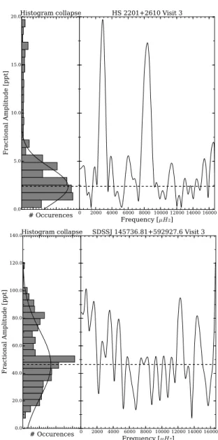
excess of a year in some cases. We decided to avoid problems associated with welding together and analyz-ing data with such large gaps in between, and instead analyze the light curves for each target on a visit–by– visit basis. Example LSPs for two of our targets are shown in the right panels of Figure2.
Candidate pulsators can be identified by comparing the highest peak in each LSP to its corresponding mean noise levelσ. While maximum peak values are simple to extract from the periodograms, mean noise levels prove to be more difficult to estimate given the short duration of each visit. Initially, the RMS scatter about the mean for each visit’s light curve was used as a mean noise level estimate – however, these values were consistently high relative to the apparent noise level (by visual in-spection) in the LSP. The poor frequency resolution in the single–visit LSPs, around∼667µHz, permits strong signals (whether real or not) to raise the estimated noise level above its actual value, thereby making the sig-nals appear at lower S/N than they are. We settled on what we found to be a relatively robust method: we “collapse” the power spectrum onto the amplitude axis, plot a histogram of amplitude values, and fit a standard Gaussian function to this distribution. We take the cen-troid of this Gaussian fit as the mean noise level for the LSP. As illustrated in the left panels of Figure 2, this method keeps noise spikes and actual stellar variations from skewing the estimated noise level, thereby permit-ting us to use the S/N of the highest peak to assess its significance properly.
Summarizing our entire data set, we plot in Figure
0 2000 4000 6000 8000 10000 12000 14000 16000
Frequency [µHz]
HS 2201+2610 Visit 3
# Occurences 0.0
5.0 10.0 15.0 20.0
Fra
cti
on
al
Am
pli
tu
de
[p
pt
]
Histogram collapse
0 2000 4000 6000 8000 10000 12000 14000 16000
Frequency [µHz]
SDSSJ 145736.81+592927.6 Visit 3
# Occurences 0.0
20.0 40.0 60.0 80.0 100.0 120.0 140.0
Fra
cti
on
al
Am
pli
tu
de
[p
pt
]
Histogram collapse
Figure 2. Lomb-Scargle periodiograms (right panels) and their projections on the amplitude axis (left panels) for example targets HS 2201+2610 Visit 3 (Top) and SDSSJ 145736.81+592927.6 Visit 3 (Bottom). The approximate mean noise level in each LSP (dashed line) is calculated from a Gaussian fit to the amplitude histogram plot.
the mean noise level. Additionally, we color each point according to the frequency associated with the highest LSP peak. Target visits with stronger photometric vari-ations will appear at larger angles off the positive hor-izontal axis (at higher σ values). The vast majority of points fall between 2σand 4σ, indicating no significant variations above the noise level.
Careful observation of Figure 3a reveals a predom-inance of visits with strong signals around 8300 µHz (∼120 s; green points) – a phenomenon which was origi-nally not expected. Investigating light curves exhibiting this signal by eye reveals a clear correlation between flux and position on the detector (“detrad”). The detrad variation and its frequency are consistent with the so–
called “petal” dither pattern of the GALEX spacecraft. In some cases, we found that this pattern even generates a false signal at its first harmonic, out near 16000µHz. Consequently, we decided to pre-whiten all light curves of this instrumental artifact. First, we fit the sum of two sine waves to each light curve, one with frequency fixed to 8341µHz and amplitude fixed to the amplitude of this signal in the LSP, and another with frequency and am-plitude fixed to those of the first harmonic of the dither pattern. The best-fitting sine waves are then subtracted from each light curve to remove the petal pattern, and new LSPs are calculated. Figure4shows the light curve and LSP for one of our target visits, before and after the pre-whitening of the petal pattern signal.
The newly pre-whitened target light curves are run through the same scripts previously discussed to gener-ate Figure3b. The predominance of points around 8000 µHz (green points) is now gone. We investigated the large number of targets remaining with maximum peak frequencies below 1000µHz (dark purple/black points) – a regime where the LSP is dominated by 1/f noise – and find that many of these visits have a long-term varia-tion introduced by a second, lower frequency spacecraft dither pattern. We elected to remove this frequency range from the calculation of the highest LSP peak for three reasons: (i) signals in this range are likely due to 1/f noise or a known, longer–period spacecraft dither pattern; (ii) these low–frequency signals can overpower true signals at other frequencies; and (iii) sdBVr pul-sations are not expected at frequencies lower than 1000 µHz anyway, so the likelihood of missing stellar pulsa-tions at f< 1000µHz is low. After this low frequency cut the most visits a target has is 119 with a mean (me-dian) of 7.4 (2) visits per target.
Figure 3c summarizes our full dataset after remov-ing or ignorremov-ing instrumental effects and 1/f noise. We present in Table1a small subset of target measurements used to produce Figure3c, with the entire set available electronically. The plot bounds of Figure3 were chosen in order to highlight the region where sdBVr pulsations are expected to exist. One will notice a sharp drop-off in point density above the 4σ line, compared to pan-els a and b (in which the dither pattern and 1/f noise dominate many LSPs). In essence, Figure 3c provides an ordered list of targets to investigate for stellar pul-sations, starting with the highest S/N objects. Before using these data to search for new pulsators, however, we attempted to recover NUV signals fromknown pul-sating sdBVr stars.
4. DETECTIONS OF KNOWN SDBVR STARS
0.0
2.0
4.0
6.0
8.0
Mean Noise Level [ppt]
0.0
20.0
40.0
60.0
Ma
xim
um
Pe
ak
[p
pt
]
2 σ
4 σ
6 σ
8 σ
A
0.0
2.0
4.0
6.0
8.0
10.0
Mean Noise Level [ppt]
2
σ4
σ6
σ8
σB
0.0
2.0
4.0
6.0
8.0
10.0
Mean Noise Level [ppt]
0.0
20.0
40.0
60.0
Ma
xim
um
Pe
ak
[p
pt
]
2
σ4
σ6
σ8
σC
4000
8000
12000
16000
Fre
que
ncy
of M
axim
um
Pe
ak [
μ
Hz]
4000
8000
12000
16000
Fre
que
ncy
of M
axim
um
Pe
ak [
μ
Hz]
Figure 3. Maximum Peak in the Lomb-Scargle Periodogram (LSP) vs. Mean Noise in the LSP. (a) - No pre-whitening, all visits plotted, (b) - pre-whitening, all visits plotted, (c) - pre-whitening, visits with a maximum peak amplitude lower than 1000µHz not plotted. Star symbols mark identified known pulsating sdBs – from left to right, HS 2201+2610 (Østensen et al. 2001), GALEX J0869+1527(Baran et al. 2011), EC 14026-2647 (Kilkenny et al. 1997), HS 0815+4243 (Østensen et al. 2001).
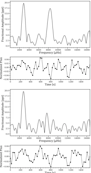
known sdBVrstars with sufficient GALEX observations for analysis, shown in Table 2, we were only able to recover pulsations in four of these objects. Their NUV light curves and corresponding LSPs are shown in Figure
5. We use non-linear, least squares fitting of sine waves to the data to determine pulsation amplitudes and fre-quencies, which are shown in Table 3. The wavelength dependence on a pulsation mode’s amplitude (especially UV–optical comparisons) has been used in the past to identify the mode’s degree indexl, among other param-eters (Randall et al. 2005). However, sdB pulsation
Visit Start Time Visit Length Mean Noise Max Peak Frequency Sigma
Target ID [#] [MJD] [s] [ppt] [ppt] [µHz]
PG 0039+049 1 54721.2825925 1059.970 1.6 285.5 704 183.9
2 54747.1058281 802.797 39.0 310.6 567 8.0
FBS 2227+383 1 55020.5734781 1129.439 10.3 541.2 809 52.6
2 55058.98114985 860.677 33.4 416.4 1057 12.5
PG 1716+426 1 55049.3895511 1644.966 3.1 111.5 616 36.4
PB 7409 1 55081.7076462 1643.916 15.5 465.1 561 30.1
2 55108.2046817 1575.557 41.0 473.4 563 11.5
Table 1. Sample results from our data analysis, showing seven GALEX visits to four sdBs with over 600s of exposure time. Mean noise, maximum peak, and frequency of maximum peak are all reported after pre-whitening for the dither pattern and the first harmonic of the dither pattern. Start Time refers to the beginning of the GALEX visit, where MJD = JD - 2400000.5
. The entirety of this table is available electronically.
0 200 400 600 800 1000 1200 1400
Time [s] −0.06
−0.04
−0.020.00
0.02 0.04
No
rm
ali
ze
d F
lu
2000 4000 6000 8000 10000 12000 14000 16000
Frequency [μHz]
0.0 2.5 5.0 7.5 10.0 12.5 15.0 17.5 20.0
Fr
ac
tio
na
l A
mp
lit
ud
e [
pp
t]
0 200 400 600 800 1000 1200 1400
Time [s] −0.04
−0.02 0.00 0.02 0.04
No
rm
ali
ze
d F
lu
2000 4000 6000 8000 10000 12000 14000 16000
Frequency [μHz]
0.0 2.5 5.0 7.5 10.0 12.5 15.0 17.5 20.0
Fr
ac
tio
na
l A
mp
lit
ud
e [
pp
t]
Figure 4. HS 2201+2610 light curve and LSP before (top) and after (bottom) pre-whitening the dither pattern alias (at≈8000µHz). We note that other features are not signif-icantly affected by the pre-whitening, most importantly the stellar pulsation near 2800µHz.
describes the distribution of powers in the LSP, after normalization by the sample variance (
Schwarzenberg-Czerny 1998). Brief comments on the four known sdBVr
stars detected are given in the sections that follow.
4.1. HS 2201+2610
From only one usable GALEX visit, we detect a single oscillation with frequency of 2800 ±45 µHz and NUV amplitude of 20±2 ppt. The optical counterpart to this signal is difficult to identify, as observations byØstensen
et al. (2001) and Silvotti et al. (2002) show that HS
2201+2610 exhibits several signals near this period with frequency separations smaller than the resolution of our periodogram. The three largest optical signals occur at frequencies 2860, 2824, and 2880 µHz, with B-filter amplitudes near 10, 4, and 1 ppt, respectively. Our detected signal is likely a blend of these, a result of our poor frequency resolution. Nonetheless, it is clear that the pulsation amplitudes in the NUV are approximately twice as high as they are in the optical. Assuming we expect a signal near 2800µHz, we calculate a 2.1×10⁻⁶ probability that a peak as large as the one observed (power∼13.1) would occur there by chance.
4.2. EC 14026-2647
The prototype pulsating sdBV star, EC 14026-2647, was originally found to be dominated by a single vari-ation of ∼12 ppt with a frequency around 6930 µHz
(Kilkenny et al. 1997). On some nights, however, a
Start Time Visit Length Mean Noise
Target ID [MJD] [s] [ppt]
PG 0911+456 53381.979664 1673.683 2.9
HS 2201+2610* 55829.740088 1582.440 2.8
PG 1657+416 52861.746673 1433.522 6.0
PG 1047+003 53092.802616 1669.538 71.5
HS 1824+5745 55820.70283 1558.150 7.2
HS 0815+4243* 55211.044285 1647.533 4.8
HS 0039+4302 53683.109493 1672.339 4.6
EC 14026-2647* 53857.464188 1693.600 4.9
GALEX J08069+1527* 55203.24052 1647.039 3.0
HE 2151-1001 54679.310077 1070.767 5.3
PG 1219+533 55633.879924 1669.925 11.9
PG 1618+562 53493.344468 1005.4 2.8
HS 2125+1105 55021.595772 887.498 23.2
Table 2. Single GALEX visit for the each of the 13 known sdBVrtargets present in our dataset. Note that the noise levels for
these targets are near to or larger than the characteristic pulsation amplitude of an sdBVr. Those targets that were identified
have pulsations amplitudes greater than the norm. * sdBVr identified in this study.
NUV Amplitude Frequency Period
Target ID [ppt] [µHz] [s]
HS 2201+2610 20±2 2800±45 357.14
EC 14026-2647 (Visit 1) 19±4 7030±75 142.24
EC 14026-2647 (Visit 2) 22±4 7074±53 141.36
GALEX J08069+1527 31±3 2810±32 355.87
HS 0815+4243 12±4 7880±121 126.9
Table 3. NUV amplitudes, frequencies, and associated uncertainties for known pulsating sdBVr stars with GALEX–detected
NUV variations.
poor noise level, bad frequency resolution, or the pulsa-tion mode simply not being present at the time of the observation is unclear.
4.3. GALEX J08069+1527
GALEX J08069+1527 had one useful GALEX visit, from which we report a single signal at 2810±32µHz with amplitude 31±3 ppt. This is a clear detection of the dominant pulsation mode reported by Baran et al.
(2011), which had aB-filter amplitude of 27 ppt. The probability this peak (power∼14.4) is due to noise alone is 5.6×10⁻⁷. We do not detect the second mode re-ported in the optical discovery data, which would have a predicted NUV amplitude below our noise level.
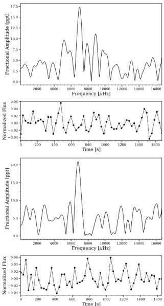
4.4. HS 0815+4243
Østensen et al. (2001) reported a signal between 5.9
and 7.8 ppt (variation over the course of three observa-tions) at a frequency of 7920µHz in HS 0815+4243. Us-ing the sUs-ingle visit available for this target, we find four peaks in the LSP that stand out above the noise level.
While the sigma value for this target is apparently quite low (especially compared to the other known pulsators identified here), it is the number of similarly large peaks – which we believe to be predominately due to noise – that serves to inflate the mean noise level thus deflating the sigma value. Consequently we see that we cannot rely solely on the sigma metric as it is subject to under estimation when the number of similarly large peaks is high. Instead this target is identified only by using prior knowledge of the pulsation. One of the large peaks, with amplitude 12±4 ppt and frequency 7880±121µHz, is consistent with theØstensen et al.(2001) detection. We find that this peak has a power of∼3.03, from which we calculate a 4.8% probability it could occur by chance.
0 200 400 600 800 1000 1200 1400 Time [s] −0.04 −0.02 0.00 0.02 0.04 No rm ali ze d F lu
2000 4000 6000 8000 10000 12000 14000 16000
Frequency [μHz]
0.0 2.5 5.0 7.5 10.0 12.5 15.0 17.5 20.0 Fr ac tio na l A mp lit ud e [ pp t]
0 200 400 600 800 1000 1200 1400 1600
Time [s] −0.050 −0.025 0.000 0.025 0.050 No rm ali ze d F lux
2000 4000 6000 8000 10000 12000 14000 16000
Frequenc [μHz]
0.0 5.0 10.0 15.0 20.0 Fr ac tio na l A mp lit ud e [ pp t]
0 200 400 600 800 1000 1200 1400 1600
Time [s] −0.050 −0.025 0.000 0.025 0.050 No rm ali ze d F lux
2000 4000 6000 8000 10000 12000 14000 16000
Frequenc [μHz]
0.0 5.0 10.0 15.0 20.0 Fr ac tio na l A mp lit ud e [ pp t]
0 200 400 600 800 1000 1200 1400 1600
Time [s] −0.075 −0.050 −0.025 0.000 0.025 0.050 No rm ali ze d F l x
2000 4000 6000 8000 10000 12000 14000 16000
Freq ency [μHz]
0.0 5.0 10.0 15.0 20.0 25.0 30.0 Fr ac tio na l A mp lit d e [ pp t]
0 200 400 600 800 1000 1200 1400 1600
Time [s] −0.04 −0.02 0.00 0.02 0.04 0.06 No rm ali e d F lux
2000 4000 6000 8000 10000 12000 14000 16000
Frequency [μH ]
0.0 2.0 4.0 6.0 8.0 10.0 12.0 14.0 Fr ac tio na l A mp lit ud e [ pp t]
Figure 5. Single–visit light curves and Lomb-Scargle periodograms for previously–known sdBVr stars detected in the GALEX
NUV data set. Clockwise from top–left, targets shown include HS 2201+2610, EC 14026-2647 Visit One, EC 14026-2647 Visit Two, GALEX J08069+1527, HS 0815+4243.
the same observation times as the GALEX light curve and inject into it Gaussian noise with variance match-ing that of the observed data set. We compute the LSP of each synthetic light curve and record its maximum power. The false alarm probability of an observed sig-nal without prior detection is equal to the fraction of trials in which the maximum power exceeds that of the observed peak. Our Monte Carlo simulations show that the three peaks at 6993, 5238, and 15368µHz have false alarm probabilities of∼30%,∼75%, and∼45%, respec-tively. Consequently, we hesitate to claim them as new detections.
5. NEW CANDIDATE PULSATING SDBS
As previously mentioned, Figure 3c and Table 1 ef-fectively provide an ordered list of targets to follow– up for confirmation of stellar pulsations. Most targets in this figure fall below the 4σ line, indicating either stellar pulsations swamped by the noise level, or the lack of pulsations altogether. Some targets, however, do show signals at higher signal–to–noise ratios. We note that many of these signals appear to be instrumen-tal in nature, remnants of poor dither-pattern subtrac-tion (green points – petal pattern fundamental
oscilla-tion; dark red points – petal pattern first harmonic). Nonetheless, a few viable targets remain at or above the 4σline and warrant follow–up observations for con-firmation. While a complete follow–up survey of these targets is beyond the scope of this paper, we were able to obtain sufficient ground–based observations of one can-didate pulsator, LAMOST J082517.99+113106.3 (SDSS J082517.99+113106.2), which we discuss in detail in the following section.
5.1. LAMOST J082517.99+113106.3 — A New sdBV
Usable GALEX data for LAMOST
J082517.99+113106.3 consists of two separate vis-its (Figure 6). Both visits reveal the same candidate signal, which has an average NUV amplitude of 19
maximize the signal–to–noise ratio so that we could easily confirm the GALEX–detected pulsation mode and look for other smaller modes that might be present. Each image had an exposure time of 20 s and cycle time of 27 s, resulting in a duty cycle near 74%.
All data were bias–subtracted, flat–fielded, and dark– subtracted using standard procedures via the Skynet pipeline. We performed aperture photometry on LAM-OST J082517.99+113106.3 using an in-house Python script. We chose the appropriate aperture radius to maximize S/N and used annuli to subtract sky bright-ness counts. Additionally, we tracked a nearby constant comparison star and ran the same aperture photometry procedure on it to remove atmospheric variations over the observing run. As with the GALEX observations, we calculated the LSP to look for any optical variations in the light curve. Figure 7 shows the resulting light curve and its amplitude spectrum. Our ground–based optical light curve reveals a photometric variation near the same frequency detected in the GALEX data. From least–squares fits of sine waves to the data, we report a “white light” amplitude of 5.4±0.8 ppt with frequency 6971±8µHz (period of 143.45±0.18 s).
Initially, we were a bit surprised at the relatively low optical amplitude of LAMOST J082517.99+113106.3. Other known sdBVs we observed had amplitudes in the optical that were approximately half that in the NUV. If LAMOST J082517.99+113106.3 followed the same trend, we would expect an amplitude of ∼10 ppt in the ground-based optical data. Further in-spection of our Skynet images revealed that LAMOST J082517.99+113106.3 had an unresolved visual compan-ion whose PSF overlapped heavily with that of the sdBV in the PROMPT-3 frames (which have a pixel scale of 1.400 per pixel). Consequently, the apertures we used when extracting photometry were heavily polluted by the companion, and our reported measurement for the optical amplitude must be underestimated. The visual companion is resolved in the Sloan Digital Sky Survey (SDSS J082518.17+113106.1) and sits∼2.700to the East
(Abazajian et al. 2009); it has SDSS colors signficantly
redder than the sdB, consistent with a late F-type or early G-type star. Such a cooler companion should be approximately 5–6 mag fainter than the sdB in the NUV (see Figure 1 ofWade et al. 2009). In this case, our NUV pulsation amplitude should be unaffected even though the pair is unresolved in GALEX. In the Skynet optical images, we used SAOImage ds9 to estimate the flux ra-tio and find that the companion is approximately 30% fainter than the sdB in the Clear filter. As such, a cor-rection factor of∼1.7 should be applied to our measured pulsation amplitude, which brings the true value closer to 9 or 10 ppt, much more consistent with the 2–to–1 ra-tio observed for the sdBV stars in Secra-tion4. LAMOST
0 200 400 600 800 1000 1200 1400 1600
Time [s] −0.04
−0.02 0.00 0.02 0.04 0.06
No
rm
ali
ze
d F
lu
2000 4000 6000 8000 10000 12000 14000 16000
Frequency [μHz]
0.0 2.5 5.0 7.5 10.0 12.5 15.0 17.5
Fr
ac
tio
na
l A
mp
lit
ud
e [
pp
t]
0 200 400 600 800 1000 1200 1400 1600
Time [s] −0.04
−0.02 0.00 0.02 0.04 0.06
No
rm
ali
ze
d F
lux
2000 4000 6000 8000 10000 12000 14000 16000
Frequenc [μHz]
0.0 5.0 10.0 15.0 20.0
Fr
ac
tio
na
l A
mp
lit
ud
e [
pp
t]
Figure 6. NUV light curve and corresponding Lomb-Scargle periodogram for LAMOST J082517.99+113106.3 Visit One (top) and Visit Two (bottom), a new candidate sdBVr star
identified from the GALEX dataset.
J082517.99+113106.3 requires higher spatial resolution follow-up in order to accurately determine a precise op-tical pulsation amplitude.
6. DISCUSSION
GALEX provides an enticing dataset to study UV– bright objects, and gPhoton makes such a study signif-icantly easier. However, the GALEX dataset is not a golden ticket for those hoping to conduct a detailed and high-resolution study of variable objects. In our work with sdBs, we identified several pitfalls when working with GALEX data queried through gPhoton that future studies should be wary of (along with those discussed
inMillion et al. 2016). First, strong detrad signals near
0 2000 4000 6000 8000 10000 12000 14000 16000 Frequency [µHz]
0.000 0.001 0.002 0.003 0.004 0.005 0.006
Fra
c i
on
al
Am
pli
ud
e
0 1000 2000 3000 4000 5000 6000 7000 8000 9000 Time [s]
−0.030 −0.0150.000 0.015 0.030
No
rm
ali
ze
d F
lux
Figure 7. Optical time–series photometry of LAMOST J082517.99+113106.3 obtained with the robotic Skynet tele-scopes. The Lomb-Scargle periodogram (top panel) reveals the presence of a∼6 ppt signal in the light curve (bottom) with frequency consistent with that found in the GALEX NUV data.
flagged as near the detector edge by gPhoton. Such instrumental signals can dominate the power in a pe-riodogram, hiding lower–amplitude stellar pulsations in their window functions. We used a pre–whitening tech-nique to remove these signals so that we could look for lower–amplitude stellar pulsations, but if any true sig-nals were present near the detrad frequencies, they were removed in the process, too.
GALEX’s observational pattern and observing ca-dence give rise to other obstacles when studying sdBVr pulsations. The typical observing run length for a sin-gle spacecraft visit was relatively short, near 25 min. The most obvious downfall of such short visits is a poor signal–to–noise level in the data; low–amplitude signals (<10 ppt) are simply difficult to detect, even for bright objects. Figure 8 shows visit–by–visit LSP noise lev-els as a function of V magnitude for the majority of our sdB targets. Even relatively bright sdBs with V = 14-15 mag have a median single–visit noise level aroundσ= 5 ppt. The 13 known pulsators extant within our dataset (Table2) give a sense of these poor noise properties; we can see that for all 13 stars the mean noise levels are near or above their charectaristic UV pulsation ampli-tudes. If one were to apply a 4σor 5σcriterion for the detection of new pulsation modes, most characteristic sdB pulsations would fall below this cutoff, masked by the noise. Another consequence of the short visit length is a less–than–desirable frequency resolution of 667µHz. While 20-25 min can be sufficient to observe at least a few cycles of even the slowest sdBVr pulsation modes, a problem arises when multiple modes are present: they easily blend together in a power spectrum, as we ob-served for HS 2201+2610.
11 13 15 17 19
Magnitude 0.0
20.0 40.0 60.0 80.0 100.0
Av
er
ag
e
V
isi
t
N
oi
se
[
pp
t]
Figure 8. Average, single–visit LSP mean noise levels for all NUV light curves, plotted against the V magnitudes of the sdB targets. Most sdBVr stars have optical amplitudes at
or below 10 ppt, an area heavily contaminated with noise.
Improvements to the signal–to–noise ratio and fre-quency resolution can be achieved through multiple vis-its to the same target. Unfortunately, few of our targets with detected pulsations had more than one visit. More-over, for those that did, GALEX’s observing pattern gives rise to large gaps between visits, sometimes on the order of years. For this reason, it is nearly impossible to combine multiple GALEX visits together for a tar-get when computing the LSP. We avoided this problem by breaking up data for each target by visit and com-puting an LSP for each visit individually; however this had the downfall of being computationally expensive, and complicating identification of pulsators as a signal would sometimes be present in some but not all visits. A few other methods for handling the breaks in data were initially considered, such as cross-correlating LSPs, or averaging LSPs together; however, due to counting and noise issues and these were rejected.
In light of the above discussion points, we consider the GALEX survey an adequate tool for identifying pulsa-tion modes in sdBVrstars in the NUV, but not charac-terizing them in detail. Large–amplitude, single–mode pulsators are an exception to this, as they are immune to GALEX’s poor single–visit frequency resolution and high noise levels.
7. CONCLUSION
We use this newfound source of data to search for short– period UV variations in all hot subdwarf stars that were observed by GALEX. While the observing cadence, visit lengths, and noise properties are less than ideal for ob-serving and characterizing sdBVrpuslations, we do de-tect UV pulsations in four previously–identified sdBVr stars and report their NUV amplitudes and frequencies. Some of our sdB targets not previously observed to vary show potential signals at the 4-σlevel or above and de-mand optical follow–up from the ground for confirma-tion. We used the robotic Skynet telescope system to obtain optical photometry of one of these candidates, LAMOST J082517.99+113106.3, and confirm its nature as a new pulsating hot subdwarf star.
The essential takeaway of our study is as follows: time–series aperture photometry can be extracted from GALEX data, but sdBs, despite being UV–bright ob-jects, are not the most ideal candidates for study with this instrument. This is due to a number of factors, foremost among them that sdB pulsation frequencies often exist very close to the dither pattern frequency
of GALEX, and sdB pulsation amplitudes are very near to the average noise level of GALEX.
ACKNOWLEDGEMENTS
This research has made use of NASA’s Astrophysical Data System. We would like to thank the Space Tele-scope Science Institute (STScI) and High Point Univer-sity (HPU) for facilitating this research. Some/all of the data presented in this paper were obtained from the Mikulski Archive for Space Telescopes (MAST). STScI is operated by the Association of Universities for Research in Astronomy, Inc., under NASA contract NAS5-26555. Support for MAST for non-HST data is provided by the NASA Office of Space Science via grant NNX09AF08G and by other grants and contracts.
Software:
gPhoton (Million et al. 2016), FaRVaE (https://github.com/tboudreaux/FaRVaE), SExtractor (Bertin & Arnouts 1996), Scipy (Jones et al. 2001), DS9REFERENCES
Abazajian, K. N., Adelman-McCarthy, J. K., Ag¨ueros, M. A.,
et al. 2009, ApJS, 182, 543
Baran, A. S., Gilker, J. T., Reed, M. D., et al. 2011, MNRAS, 413, 2838
Barbary, K. 2016, The Journal of Open Source Software, 1, doi:10.21105/joss.00058
Bertin, E., & Arnouts, S. 1996, A&AS, 117, 393
Brown, T. M., Ferguson, H. C., Davidsen, A. F., & Dorman, B. 1997, ApJ, 482, 685
Geier, S., Østensen, R. H., Nemeth, P., et al. 2016, ArXiv e-prints, arXiv:1612.02995
Geier, S., Marsh, T. R., Wang, B., et al. 2013, A&A, 554, A54 Han, Z., Podsiadlowski, P., Maxted, P. F. L., & Marsh, T. R.
2003, MNRAS, 341, 669 Heber, U. 2016, PASP, 128, 082001 Kilkenny, D. 2010, Ap&SS, 329, 175
Kilkenny, D., Koen, C., O’Donoghue, D., & Stobie, R. S. 1997, MNRAS, 285, 640
Lomb, N. R. 1976, Ap&SS, 39, 447
Martin, D. C., Fanson, J., Schiminovich, D., et al. 2005, ApJL, 619, L1
Million, C. C., Fleming, S. W., Shiao, B., et al. 2016, gPhoton: Time-tagged GALEX photon events analysis tools,
Astrophysics Source Code Library, , , ascl:1603.004 Millman, K. J., & Aivazis, M. 2011, Computing in Science &
Engineering, 13, 9
Moni Bidin, C., Catelan, M., Villanova, S., et al. 2008, in Astronomical Society of the Pacific Conference Series, Vol. 392, Hot Subdwarf Stars and Related Objects, ed. U. Heber, C. S. Jeffery, & R. Napiwotzki, 27
Morrissey, P., Conrow, T., Barlow, T. A., et al. 2007, ApJS, 173, 682
Oliphant, T. E. 2007, Computing in Science and Engg., 9, 10 Østensen, R., Solheim, J.-E., Heber, U., et al. 2001, A&A, 368,
175
Østensen, R. H., Telting, J. H., Reed, M. D., et al. 2014, A&A, 569, A15
Østensen, R. H., Oreiro, R., Solheim, J.-E., et al. 2010, A&A, 513, A6
Randall, S. K., Fontaine, G., Brassard, P., & Bergeron, P. 2005, ApJS, 161, 456
Reichart, D., Nysewander, M., Moran, J., et al. 2005, Nuovo Cimento C Geophysics Space Physics C, 28, 767
Scargle, J. D. 1982, ApJ, 263, 835
Schwarzenberg-Czerny, A. 1998, MNRAS, 301, 831
Silvotti, R., Janulis, R., Schuh, S. L., et al. 2002, A&A, 389, 180 Wade, R. A., Stark, M. A., Green, R. F., & Durrell, P. R. 2009,