SOURCE MECHANISM OF VOLCANIC EXPLOSIONS
INVESTIGATED BY SEISMO-ACOUSTIC
OBSERVATIONS
Keehoon Kim
A dissertation submitted to the faculty of the University of North Carolina at Chapel Hill in partial fulfillment of the requirements for the degree of Doctor of Phi-losophy in the Department of Geological Sciences.
Chapel Hill 2013
Approved by:
Dr. Jonathan M. Lees
Dr. Lara S. Wagner
Dr. Jose A. Rial
Abstract
KEEHOON KIM: Source Mechanism of Volcanic Explosions Investigated by Seismo-Acoustic Observations
(Under the direction of Dr. Jonathan M. Lees)
Source mechanisms of explosive, volcanic eruptions are critical for
understand-ing magmatic plumbunderstand-ing systems, determinunderstand-ing the evolution and geometry of source
regions, and assessing eruptive behavior as well as hazard impact. In the last two
decades, volcano seismo-infrasonic observations have become an essential part of
vol-cano monitoring systems. Because the open vent of a volvol-cano is a corridor connecting
the solid earth to the atmosphere, explosive eruptions efficiently excite both
infra-sound and seismic waves. Each of these mechanical waves includes characteristic
information on several stages of the eruption process, and the coupling of these
pro-cesses sheds considerable light into volcano dynamics. In this dissertation, details of
the explosive eruption mechanism are investigated by seismo-acoustic observations at
two volcanoes: Karymsky Volcano in Kamchatka, Russia, and Tungurahua Volcano,
Ecuador. First, path effects of infrasound waves near volcanic craters are investigated
as they pass the rim of the vent and propagate to remote stations. Next,
character-istics of infrasonic sources excited by volcanic explosion are explored. Distortion due
to diffraction and reflection of infrasound at the crater vent is shown to be
signifi-cant and must be accounted for when interpreting explosion source physics from wave
fields. To address these problems we propose an acoustic, multipole source model in
a half-space for volcanic explosions. Acoustic observations at Tungurahua Volcano
Using this approach, the time evolution and geometric orientation of the magmatic
plumbing system, during a period of volcanic crises at Tungurahua, are illuminated
Dedication
Acknowledgements
I would like to thank Dr. Jonathan Lees for his guidance during my Ph. D.
research. He has been an excellent mentor as well as a good friend. I also would
like to thank all members of the seismology group in the Department of Geological
TABLE OF CONTENTS
List of Tables . . . ix
List of Figures . . . x
1 Infrasonic wavefields excited by volcanic explosions . . . 12
1.1 Abstract . . . 12
1.2 Introduction . . . 12
1.3 Data Acquisition . . . 13
1.4 FDTD propagation model . . . 14
1.5 Results . . . 16
1.6 Discussion and Conclusion . . . 18
2 Volcanic infrasound source model . . . 24
2.1 Abstract . . . 24
2.2 Introduction . . . 25
2.3 Monopole and dipole source models in a free-space . . . 27
2.3.1 Monopole source . . . 28
2.3.2 Dipole source . . . 30
2.4.2 Dipole source . . . 34
2.5 Inversion for source parameters . . . 36
2.6 Stability of inversion method . . . 39
2.7 Infrasound radiation pattern and source characteristics . . . 43
2.7.1 Field experiment . . . 43
2.7.2 Inversion for source parameters . . . 44
2.7.3 Results . . . 48
2.8 Discussion . . . 52
2.8.1 Direct Sources . . . 53
2.8.2 Diffraction and Reflection . . . 53
2.8.3 Aerodynamic Flow . . . 56
2.9 Conclusion . . . 59
3 Source mechanism of Vulcanian eruption. . . 60
3.1 Abstract . . . 60
3.2 Introduction . . . 61
3.3 Tungurahua Volcano and Seismo-Acoustic Data . . . 63
3.4 Moment Tensor Inversion . . . 69
3.5 Result . . . 71
3.5.1 Squared Error . . . 71
3.5.2 Source Location and Source Time Function . . . 72
3.5.3 Resolution of Single Forces . . . 73
3.6 Discussion . . . 85
3.6.1 Geometry of Source Region . . . 85
3.6.2 Time Histories of Source Processes . . . 89
3.7 Conclusion . . . 93
LIST OF TABLES
1.1 Modeling Parameters . . . 17
2.1 Estimates of the source parameters . . . 42
2.2 Statistics of the source parameters . . . 45
3.1 Residual errors and Akaike’s Information Criterion . . . 72
LIST OF FIGURES
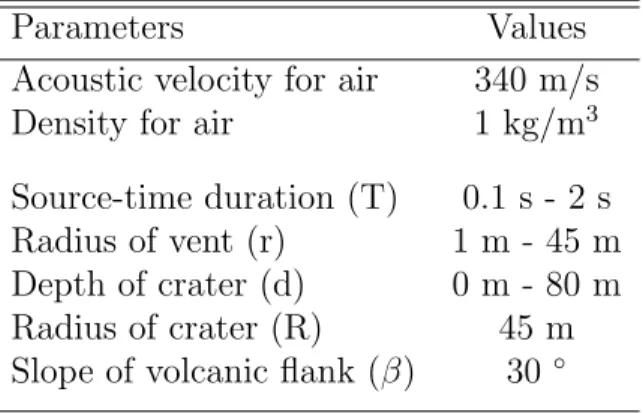
1.1 Map of Karymsky volcano and modeling parameters . . . 21
1.2 Modeling results . . . 22
1.3 Comparison between model and observations . . . 23
2.1 Geometric configurations for monopole and dipole . . . 29
2.2 Theoretical directivity patterns for far-field sound radiation . . . 35
2.3 Comparison of Trial 1 and 4 . . . 40
2.4 Map of Tungurahua volcano with the station geometry. . . 46
2.5 Data fitting and estimated source parameters . . . 47
2.6 Estimated source parameters using events at Tungurahua . . . 48
2.7 Crater geometry of Tungurahua volcano . . . 49
2.8 Configuration for FDTD modeling . . . 57
2.9 Comparison between the diffraction and the multipole patterns . . . . 58
3.1 Map of Tungurahua volcano with the station geometry . . . 64
3.4 Particle motions observed on the network . . . 67
3.5 Seismic signals recorded during the eruption period . . . 68
3.6 Best-fit source location of Event 1 . . . 74
3.7 Waveform fit for Event 1 listed in Table 3.2 . . . 75
3.8 The source time functions of Event 1 for Model 1 . . . 76
3.9 Three-dimensional representation of the eigenvectors . . . 77
3.10 Source time functions of Event 1 obtained by assuming Model 2 . . . 77
3.11 Numerical test of the capability of the inversion method . . . 78
3.12 Source type plot of Hudson et al. (1989) . . . 80
3.13 The eigenvectors of the moment tensors . . . 81
3.14 Ratios of eigenvalues . . . 86
3.15 Resultant ellipsoidal cavity obtained from the mean eigenvectors . . . 87
CHAPTER 1.
Infrasonic wavefields excited by volcanic explosions
1.1
Abstract
Numerical modeling of waveform diffractions along the rim of a volcano vent shows
high correlation to observed explosion signals at Karymsky Volcano, Kamchatka,
Russia. The finite difference modeling assumed a gaussian source time function and
an axisymmetric geometry. A clear demonstration of the significant distortion of
infrasonic wavefronts was caused by diffraction at the vent rim edge. Data collected
at Karymsky in 1997 and 1998 were compared to synthetic waveforms and variations
of vent geometry were determined via grid search. Karymsky exhibited a wide range
of variation in infrasonic waveforms, well explained by the diffraction, and modeled
as changing vent geometry. Rim diffraction of volcanic infrasound is shown to be
significant and must be accounted for when interpreting source physics from acoustic
observations.
1.2
Introduction
In the last 10 years infrasonic acoustic waves have played an increasingly important
mic recordings of volcanic explosions, infrasound has a simplified Green’s function
and can thus provide a direct measure of physical source dynamics in the vicinity of
the volcanic vent. Signals in the infrasonic frequency band (< 20 Hz) (Wilson and
Forbes, 1969; Kanamori et al., 1994) can have several sources, and explicit wave
sim-ulation is required to extract and separate source dynamics from propagation effects.
Although infrasonic waves are not as affected by path effects at short source-receiver
distances, the distorting effects of vent geometry and atmospheric perturbation must
be considered and removed in order to understand the underlying source dynamics of
individual explosions.
We focus here on the volcanic vent geometry and its effect on infrasonic waveforms
generated near the source during volcanic eruptions. When in close proximity to a
volcano source (<10 Km) propagation paths can be approximated by straight lines
and atmospheric refraction and reflection distortion are, for the most part,
negligi-ble (Johnson et al., 2006; Ripepe et al., 2007). Here we model infrasound wavefields
passing through a volcanic vent with varying radii and compare them with
obser-vations from Karymsky volcano, Russia. Wavefront deformation through the vent
and past the rim is shown to be considerable and in significant agreement with field
observations. We attribute the wave distortion to diffraction at the edge of the vent.
1.3
Data Acquisition
Karymsky Volcano is a 1540-m andesitic cone located in the central portion of
Kam-chatka’s main active arc in Russia. Seismo-acoustic data presented here were collected
at Karymsky volcano during two field surveys in August 1997 and September 1998
(Johnson et al., 2003; Lees et al., 2004). In 1997 and 1998, Karymsky exhibited long
periods of discrete Strombolian explosive activity with a repetitive explosions ranging
PASS-CAL Reftek A-07 and A-08 dataloggers with 3-component broadband seismometers
and microphones on the lower flanks of the volcano, at distances 1500 - 5000 m from
the summit crater (Figure 1.1a). In 1998, a microphone equipped with the
Larsen-Davis 2570 electret condenser was used with laboratory-calibrated single-pole corner
frequency at 0.27 Hz (3 dB down) and nominal sensitivity of 48 mV/Pa (Johnson,
2007). In 1997, however, a different electret condenser-based microphone was
de-ployed (Johnson et al., 2003; Ripepe et al., 2007). The 1997 microphone was found
to be sensitive to changes in pressure rather than absolute pressure, so measures of
the time-derivative of pressure are recorded in the field. The electret condenser
mi-crophone has a flat response function in the audible band (20 Hz - 20 KHz), however
calibration and sensitivity below 20 Hz is unavailable at this time, so detailed
decon-volution is not possible. Since the signal-to-noise ratio for both 1997 and 1998 data
are high and observations are in such good agreement with synthetic modeling, we
present results from the 1997 modeling as corroboration of our approach in spite of
the lack of calibration.
Among thousands of events recorded, 214 explosions (134 from 1997 and 80 from
1998) were selected for comparison to synthetic wave propagation modeling. Criteria
for selection included: (1) impulsive, short duration signals (< 10 s) and (2) high
signal-to-noise ratio (28±9 dB) below 10 Hz. We thus avoid signals whose waveforms
potentially interact with conduit walls and the fluid/air interface.
1.4
FDTD propagation model
A Finite-Difference Time-Domain (FDTD) method was used to synthesize acoustic
wave propagation formulated as a set of first-order, velocity-pressure coupled
atmosphere and the ground (de Groot-Hedlin, 2008). To approximate the derivatives
in the acoustic wave equation with finite differences, a staggered difference algorithm
(Yee, 1966) was used in a two-dimensional cylindrical spatial domain. Time marching
was staggered between the computations of pressure and particle velocity in the time
domain. By restricting the computation to an axisymmetric cylindrical
representa-tion (volcanic cone and vent) calcularepresenta-tions can be performed quickly on a desktop
computer.
The perfectly matched layer technique (Berenger, 1994; Liu, 1999) was adapted for
absorbing boundary conditions achieving highly effective suppression of reflections at
the domain boundaries. In order to examine effects of ground surface and topographic
reflections, diffractions, and scattering by the volcano geometry, a rigid boundary
condition between the air and solid surface was implemented via the method of images
(Morse and Ingard, 1986). Intrinsic attenuation and moving media are ignored in
this simulation. In order to reduce numerical errors arising from the “staircase”
representation of the rigid boundary, the model is spatially discretized using 20 grid
points per wavelength, double the recommended minimum of 10 (Wang, 1996).
The volcanic conduit was modeled as an air-filled cylinder buried in a rigid
vol-canic cone, where the atmosphere was treated as a fluid halfspace connected to the
magmatic system through the open vent (Figure 1.1b). In real volcanic environments,
the conduit is likely filled with multi-phase fluids consisting of air, gas, and magma.
In this study we simply assume that the top of the conduit consists of constant 340
m/s velocity air. Inhomogeneities and wind in the atmosphere, nonlinear behavior,
and the effects of gravity are ignored. Supersonic flux of the initial mass and very
large pressure purtubations (> 103P a) can cause non-linear shock waves.
Strom-bolian ejection velocities, however, generally range up to a few hundred meters per
second (Sparks, 1997). Source pressures calculated from Karymsky data do not
linearized acoustic equation. Because our aim is to investigate deformation of
wave-fronts passing through the vent, longitudinal reflection at the air-magma interface
is suppressed by incorporating an absorbing boundary at this interface, preventing
down-going waves from being reflected back towards the summit.
The average outer radius of the active crater remained mostly constant at 45
meters from 1996 to 1998 based on geodetic observations (Alexei Ozerov, personal
contact). Inner vent radius, depth and source frequency were allowed to vary as model
parameters (Table 1.1).
The direct source of volcanic infrasound is atmospheric vibration at the air-magma
interface. This perturbation can be generated by mass outflux through, or
accelerat-ing movement of, the interface. We use mass outflux here as the source because we
have observed, visually, gas emission associated with infrasonic events. High
ampli-tude infrasound is more effectively excited by explosive gas emission than by large
displacement of the air-magma interface (Johnson et al., 2004). Mass flux is assumed
here to be spatially constant over the air-magma interface, exciting only the plane
wave mode in the conduit. The plane wave condition is not exact, as real volcanic
sources most probably simultaneously excite radial modes. The conduit walls act as
waveguides, however, preventing the low frequency radial modes from being
gener-ated. Therefore, the plane wave is the predominant mode in the conduit as long as
the vent radial dimension is smaller than the source wavelength. A gaussian-shaped
pulse (Blackman-Harris window function) was used as the source-time-function for
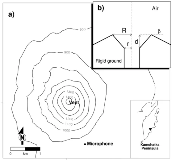
the mass flux (Figure 1.2c).
1.5
Results
Table 1.1: Modeling Parameters illustrated in Figure 1.1b
Parameters Values
Acoustic velocity for air 340 m/s Density for air 1 kg/m3
Source-time duration (T) 0.1 s - 2 s Radius of vent (r) 1 m - 45 m Depth of crater (d) 0 m - 80 m Radius of crater (R) 45 m Slope of volcanic flank (β) 30◦
vent. Sound propagation excited by a vibrating piston buried in the rigid halfspace
has been widely studied in the field of acoustics (Harris, 1981). Briefly, acoustic
wavefronts of overpressure from a vibrating piston are composed of two components:
a plane “direct wave” generated by vertical piston movement propagating along the
conduit axis, followed by spherical, “edge waves”, produced by diffraction along the
vent edge (Figure 1.2a). In the cylindrical region immediately above the vent, the
consequent wavefront consists of a direct wave followed by edge waves. Outside the
cylindrical region, however, two edge waves with opposite polarities are the major
contributors to the wavefield (Weight and Hayman, 1978).
In most exploding volcano situations, for reasons of safety, receivers are restricted
to flanks away from the vent rim, and edge effects contribute considerably to observed
signals. If the source is impulsive (Figure 1.2c), the two inverted pulses are readily
observed on real recordings (Figure 1.2d). The lag and amplitudes of the two inverted
pulses are constrained by the conduit radius, assuming the radius is constant with
depth. In our modeling domain, however, acoustic waves are affected by diffraction
from the edge of the inner and outer apertures of the crater. In Figure 1.2a and
1.2b, two diffractions are illustrated. When the original waves emanate from the
inner vent, they diffract and the diffracted waves oscillate horizontally inside the
vent radii and the associated crater depth.
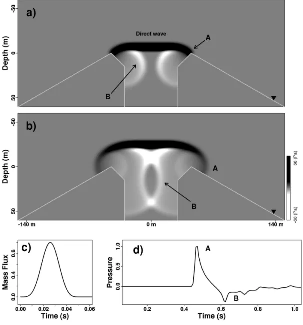
Figure 1.3 shows a series of transient acoustic waveforms deformed by different
geometries and different source-time-functions. The waveform distortion from the two
edge waves with opposite polarities is clear, and sensitive to the geometry of the vent.
These synthetic waveforms were compared to real data observed at Karymsky and the
fit is extremely good (>0.83 cross-correlation values for 90% of events). One series of
observations which illustrate the waveform dependency on the vent geometry and the
source time duration is illustrated in Figure 1.3. Impulsive explosions and subsequent
oscillations were successfully reproduced by numerical modeling. Numerical modeling
indicates that diffraction at the vent edge plays a significant role in the observed
waveforms.
1.6
Discussion and Conclusion
Based on the theory of acoustic radiation from a vibrating piston, the contribution
of diffracted edge waves to the wavefield depends on the vibration velocity and the
diameter of the piston. If the wavelength of the vibration is much larger than the
piston diameter, the larger of the two edge waves overlaps such that the radiating
pressure waves are proportional to the time derivative of the vibration velocity, i.e. the
acceleration. In this limit, the piston corresponds to a point source radiator. On the
other hand, if the velocity wavelength is shorter than the piston diameter, two edge
waves can be resolved without overlap. In this case, each edge wave closely resembles
(slightly dispersed) the vibration velocity rather than the acceleration (Weight and
Hayman, 1978). Infrasound data recorded in the field at Karymsky exhibit this
diffraction phenomenon. When the source wave length (265 m) is larger than the
is almost the same as that of the source time function representing mass flux. When
the source wavelength (64 m) is shorter than the crater, however, the two edge waves
can be separated such that the first arrived edge wave is highly correlated to the mass
flux function (bottom panel, figure 1.3a) . The latter edge wave is more attenuated
and may be contaminated by reverberations within the crater. This dependency on
vent dimensions and source wavelength was observed also in 1997 (figure 1.3b) where
the instrument recorded the time-derivative pressure field (Ripepe et al., 2007).
The assumption of a gaussian shaped source function and plane waves appears to
be justified by the excellent correlation of model results with field observations. First,
because only short duration pulses were selected from the Karymsky data, sources
must be simple. Second, the vent wall behaves as a waveguide and the plane wave
dominates even though the source wavelength is slightly shorter than or equal to the
vent diameter. Third, the real source may have a vertical component amplitude larger
than the radial component. The true directivity of the source can not be estimated
without observations of the direct wave (as defined previously) above the vent or
refracted in the far field.
We focused here primarily on the presence of edge waves near a volcanic crater
and on how they are related to source waveforms. A more detailed study may provide
insight to the relation of the time lag (∆t) between edge waves and the vent geometry,
although that is beyond the scope of this paper. The time lag has a strong dependence
on the source waveform and vent geometry, however, if the pulse wavelength is shorter
than the vent diameter (bottom, figure 1.3a), the two edge waves do not overlap and
the time lag can be reduced to a function of geometric parameters alone. In the case
of a simple piston with constant radius, this time lag corresponds only to the piston
diameter (Weight and Hayman, 1978). However, in our model with varying radii,
the time lag depends on the inner vent radius and the depth as well as the outer
geometric features of the vent.
FDTD modelings of infrasonic observations from Karymsky volcano showed that
the wavefields in the near field are significantly affected by diffraction. The
morphol-ogy of the crater plays an essential role in waveform distortion. Our results show that
it is critical to take diffraction effects into account when interpreting source physics
CHAPTER 2.
Volcanic infrasound source model
2.1
Abstract
Volcanic explosions are accompanied by strong acoustic pressure disturbances in the
atmosphere. With a proper source model, these acoustic signals provide invaluable
information about volcanic explosion dynamics. Far-field solutions to volcanic
infra-sound radiation have been derived above a rigid half-space boundary, and a simple
in-version method was developed based on the half-space model. Acoustic monopole and
dipole sources were estimated simultaneously from infrasound waveforms. Stability of
the inversion procedure was assessed in terms of variances of source parameters, and
the procedure was reliable with at least three stations around the infrasound source.
Application of this method to infrasound observations recorded at Tungurahua
vol-cano in Ecuador successfully produced a reasonable range of source parameters with
acceptable variances. Observed strong directivity of infrasound radiation from
explo-sions at Tungurahua are successfully explained by the directivity of a dipole source
model. The resultant dipole axis, in turn, shows good agreement with the opening
direction of the vent at Tungurahua which is considered to be the origin of the dipole
2.2
Introduction
Volcanic eruptions are efficient sources of atmospheric pressure perturbations within
the infrasound band (<20 Hz). Volcanic infrasound is a direct measurement of
fluc-tuation at the magma-air interface, and the atmosphere in the vicinity of the vent
has a relatively simple Green’s function compared to the solid medium through which
seismic waves propagate. Hence, volcanic infrasound can carry valuable information
about source dynamics without significant loss of source features compared to the
seismic counterpart (Vergniolle et al., 1996; Garces and McNutt, 1997; Ozerov et al.,
2003; Johnson and Lees, 2010).
A proper acoustic source model is necessary to extract the underlying physics of
volcanic eruptions from infrasound observations. Real acoustic sources producing
vol-canic infrasound have finite dimensions such as radius of bubble or vent. In this case,
source geometry and frequency dependent diffraction must be considered (Kim and
Lees, 2011). However, if the source region is compact with respect to the wavelength,
then the source can be dealt with as a point with magnitude but no spatial dimension.
This point source approximation has been widely used in volcanic infrasound studies
to quantify acoustic energy produced during volcanic eruptions (Johnson et al., 2004;
Johnson, 2007; Ripepe et al., 2007; Vergniolle et al., 2004).
A monopole is the simplest and most efficient point source of volcanic infrasound.
Sound generated by a monopole radiates uniformly into all directions. Isotropic mass
outflux during volcanic eruptions can be modeled as a monopole source, and volume
or velocity of ejecting material can be estimated from acoustic pressure (Woulff and
McGetchin, 1976; Johnson et al., 2004).
Forces generated during volcanic activity can be simulated by a dipole source,
which has two successive monopoles out of phase by 180◦. Pressure disturbance by
angle between the direction of the dipole and station location. Caplan-Auerbach et al.
(2010) used acoustic power observed at Augustine volcano, Alaska, to estimate the
velocity of material exiting the vent based on the dipole model.
In both cases, selecting a proper source model is critical for estimating energy
flux in the vicinity of a volcanic vent. Most studies of volcanic infrasound have
used either a monopole or dipole source exclusively to model acoustic sources of
volcanic eruptions, but theoretically both types of acoustic sources can be excited
simultaneously. For instance, an unbaffled loudspeaker is theoretically an ideal dipole
source. However, sound measurements from the loudspeaker are not explained solely
by the dipole model, and the substantial monopole component is also required (Li
et al., 1997). Hence, “multipole” sources can be appropriate for acoustic sources of
volcanic infrasound.
In this paper we review the solutions to the scalar wave equation for monopole
and dipole sources in a half-space, and then present an inversion method based on
the half-space model to estimate source parameters for a monopole and dipole
simul-taneously. The inversion method is applied to infrasound observations from
Tungu-rahua volcano, Ecuador in 2010 which exhibited remarkable directivity in acoustic
radiation. The inversion process successfully estimated stable and consistent source
parameters corresponding to the recorded radiation patterns. Consequently, the
in-frasound radiation pattern observed at Tungurahua volcano is well explained by the
multipole source. The dipole component contributes to the observed directivity, and
the monopole does to the overall pressure level. The multipole source model in a
half-space gives us a powerful method to cope with complicated sources for volcanic
2.3
Monopole and dipole source models in a
free-space
Acoustic radiation fields from sources of limited spatial extent can be described in
terms of a multipole series. If the source is acoustically compact, so that its largest
dimension is much shorter than a wavelength, the multipole series converges rapidly
and the first few terms remain nonzero. Consequently, compact sources are typically
approximated as monopole, dipole, and quadrupole terms (Rossing, 2007) although
only monopole and dipole cases are considered in this paper. It is convenient to write
the total sound field in terms of a Green’s function. Assuming a point source placed
atr0 = (x0, y0, z0) in an unbounded atmosphere, the total sound field p(r, t) satisfies the inhomogeneous wave equation
∇2p− 1
c2
∂2p
∂t2 =−δ(t)δ(r−r0), (2.1)
where p is pressure, c is the sound speed, and r = (x,y,z) is a receiver position. If the source is simple-harmonic, so that δ(t) from the origin can be substituted by
e−iωt the resulting wave motion is p = ˆp(ω)e−iωt, which satisfies the inhomogeneous
Helmholtz equation
∇2pˆ(ω) +k2pˆ(ω) =−δ(r−r
0). (2.2)
The Green’s function solution to the Helmholtz equation (Morse and Ingard, 1986) is
Gω(r|r0) = 1 4πRe
ikR, (2.3)
frequencies, as follows:
G(r, t|r0, t0 = 0) = Z ∞
−∞
Gω(r|r0)e−iωtdω
= Z ∞
−∞
1 4πRe
−iω(t−R/c)dω
= δ(t−R/c)
4πR . (2.4)
G(r, t|r0, t0) is the Green’s function for Eq. (2.1), and Gω(r|r0) can be interpreted as the Fourier transform pair of G(r, t|r0, t0). Expressions for monopole and dipole sources can be derived subsequently from the Green’s function.
2.3.1
Monopole source
A point monopole is the simplest source for sound (Fig. 2.1a). Consider the radiation
from a pulsating sphere with a small radius. If the mass flow of fluid from the source
isS(t), which is called the monopole strength hereafter, the excess pressure radiated
from a monopole can be expressed as (Morse and Ingard, 1986)
∇2p− 1
c2
∂2p
∂t2 =−S˙(t)δ(r−r0), (2.5)
where ˙S(t) is the mass flow rate per unit time, or mass acceleration in units of
ρm3/s2 where ρ is the fluid density in kg/m3. If the source is harmonic such as
S(t) = ˆS(ω)e−iωt, the solution can be expressed in terms of the Green’s function (Eq.
2.3)
ˆ
p(ω) = −ikcSˆ(ω)Gω
= −ikcSˆ(ω)
4πR e
ikR
x
z
r
0r
R
+
a)
x
z
+
−
d
r
0r
R
θ
b)
x
z
z
0z
0r
R
R'
+
+
Air Rigid bodyθ
c)
x
z
z
0z
0r
R
R'
+
−
+
−
Air Rigid bodyθ
d)
The transient solution becomes
p(r, t) = Z ∞
−∞
ˆ
p(ω)e−iωtdω
= 1
4πR
˙
S(t− R
c). (2.7)
The pressure at any point r in the field is omni-directional and determined by the mass acceleration ˙S(t) of the simple source. A body of oscillating volume, such as a
boxed loudspeaker at low frequencies, is a good example of a monopole source.
2.3.2
Dipole source
In order to generate the sound field from a point monopole, fluid must be introduced
or withdrawn from a small region of space. In the dipole case sound can be produced
by moving a portion of the fluid back and forth with no net introduction of fluid.
The dipole source is simulated by a neighbouring pair of equal point monopoles with
opposite signs. In this way fluid is being “breathed in” by one source as it is being
“breathed out” by the other source. If the source of strength S(t) is at r0 +12d and the one of strength −S(t) is at r0 − 12d, and the vector distance (d) between the two sources (Fig. 2.1b) is very small compared with the wavelength, then the wave
equation for the dipole source can be expressed as (Morse and Ingard, 1986)
∇2p− 1
c2
∂2p
∂t2 = ∇ ·[ ˙S(t)dδ(r−r0)]
= −D(˙ t)· ∇0δ(r−r0). (2.8)
D(t) = ˆD(ω)e−iωt,
ˆ
p(ω) = −ikcD(ˆ ω)· ∇0Gω(r|r0) = − k
2c
4πR
1 + i
kR
eikR×
(x−x0)
R
ˆ
Dx+
(y−y0)
R
ˆ
Dy +
(z−z0)
R ˆ Dz . (2.9)
In the far field where the distance is much longer than the wavelength, the condition,
kR 1, is satisfied. Furthermore, if r0 = 0 so that |r| =R = r, equation (2.9) can be approximated as
ˆ
p(ω) ' −k
2c 4πr
hx
rDˆx+ y rDˆy+
z rDˆz
i
eikR (2.10)
= −k
2c
4πr|Dω|cosθe
ikR, (2.11)
whereθ is the angle between the dipole vector and thez coordinate axis (Fig. 2.1b).
The sound field generated by the dipole shows directivity which depends on the angle
θ. The magnitude of the pressure disturbances is maximum on the dipole axis, and
zero at 90◦. This dipole solution can be separated into two components: the vertical
and horizontal. Any arbitrary dipole can be decomposed into vertical and horizontal
dipoles and the sound field can be rewritten, as follows:
ˆ
pH(ω) = −k
2c 4πr
hx
rDˆx+ y rDˆy
i
eikR, (2.12)
ˆ
pV(ω) =−k
2c 4πr hz r ˆ Dz i
eikR, (2.13)
where ˆpH(ω) and ˆpV(ω) are the sound fields generated by the horizontal and vertical
dipole, respectively. By considering the vertical and horizontal dipole components
of the total sound field independently, it is easier to establish the effects of a solid
2.4
Monopole and dipole source models in a
half-space
In the far-field, volcanic infrasound can be considered to propagate in a half-space.
In this range and at low frequencies, irregular topography can be ignored so that the
solid boundary can be approximated as being flat. Even though the ground surface
absorbs some acoustic energy, especially in the high frequency range, it is assumed
to be a rigid boundary due to a high contrast in acoustic velocity. If the plane is
perfectly rigid, then the boundary condition requires that the normal fluid velocity
is zero at the surface. This boundary condition can most easily be met using the
image method. An image, S0, having the same phase and magnitude as the source,
S, is placed a distance z0 below the boundary, and the boundary is removed. In
other words the rigid part is replaced by air (Fig. 2.1c). The resulting sound waves
generated by both source and image radiate into unbounded space satisfying the
boundary condition. Naturally, only the region above the boundary plane contains
the medium and carries acoustic energy. Conversely, the region below the boundary
has no physical reality. Mathematically, the wavefield reflecting from the rigid plane
represents the superposition of two wavefields generated by both source and image.
Hence, the Green’s function for a half-space can be written in terms of two Green’s
functions in a free space (Morse and Ingard, 1986)
gω(r|r0) = Gω(r|r0) +Gω(r|r00), (2.14)
2.4.1
Monopole source
Monopole radiation in a half-space can be easily solved by replacing the Green’s
function, Gω in Eq. (2.6) with gω
ˆ
p(ω) = −ikcSˆ(ω)gω(r|r0)
= −ikcSˆ(ω) [Gω(r|r0) +Gω(r|r00)] = −ikcSˆ(ω)
1 4πRe
ikR+ 1
4πR0e
ikR0
. (2.15)
At distances R from the source, which are much larger than the source is from the
origin (i.e., for Rr0), the two waves combine to form what appears to be a single,
non-simple source at the origin. When rr0 and r0 = (0,0, z0),
R = |r−r0| 'r−z0cosθ,
R0 ' r+z0cosθ, (2.16)
then,
ˆ
p(ω) ' −ikcSˆ(ω)
2πr cos(kz0cosθ)e
ikr
' −ikcSˆ(ω)
2πr e
ikr (if kz
0 1). (2.17)
If kz0 1, i.e. if the location of the source above the boundary is considerably
less than a wavelength, the far field is very weakly dependent on θ, thus resembling
the far field from a simple source with strength 2 ˆS(ω) at the origin. The effective
strength is doubled because the reflected wave adds to the initial wave in this case;
double strength. The transient solution (Lighthill, 1978) in the time domain becomes
p(r, t) = 1 2πr
˙
S(t−r
c). (2.18)
2.4.2
Dipole source
As in the monopole case, dipole radiation in a half-space can be obtained from the
Green’s function shown in Eq (14). If the source at z0 is a dipole of strength ˆD(ω) inclined at angle θ with respect to the vertical axis, then the mirror image will have
the same x and y components as the source, but a Dz opposite in sign from that of
the source. Therefore the total sound field is
ˆ
p(ω) = −ikcD(ˆ ω)· ∇0gω(r|r0)
= −ikcD(ˆ ω)· ∇0[Gω(r|r0) +Gω(r|r00)] (2.19)
Using the same approximations for R and R0, and kr 1 the far field solution can
be obtained as (Morse and Ingard, 1986)
ˆ
p(ω) ' −k
2c
2πr
hx
r
ˆ
Dx+
y r
ˆ
Dy
cos (kz0cosθ)− i
z r
ˆ
Dzsin (kz0cosθ) i
eikr
= −k
2c
2πr
hx
r
ˆ
Dx+
y r
ˆ
Dy
− iz r
ˆ
Dzkz0cosθ i
eikr (2.20)
It is convenient to split the sound fields into two parts corresponding to the horizontal
(ˆpH) and vertical dipole (ˆpV) sources
ˆ
pH(ω) = −
k2c 2πr
x
r
ˆ
Dx+
y r
ˆ
Dy
eikr (2.21)
= −k
2c
4πrDˆHcosφe
90° 0° 90° ● ● ● ● ● ● ● ● ● ● ● ● ● ● ● ● ● ● ● ● ● ● ● ● ● ● ● ● ● ● ● ● ● ● ● ● ●
a)
Free−space●●● Half−space
+
−
0° 90° 180° ● ●●●●●●●● ●●● ●● ● ● ● ● ● ● ● ● ● ● ● ● ● ● ● ● ● ● ● ● ● ● ● ● ● ● ● ● ● ● ● ● ● ● ● ● ● ● ● ● ● ● ● ● ● ● ● ● ● ●● ●●●●●●●b)
Free−space●●● Half−space
+
−
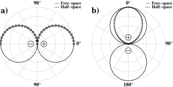
Figure 2.2: Theoretical directivity patterns for far-field sound pressure radiation from (a) horizontal dipole (Eq. 2.12 and 2.21) and (b) vertical dipole (Eq. 2.13 and 2.23). Pressures are normalized to their own maximum amplitudes.
ˆ
pV(ω) = ik 3c
2πr
z
r
ˆ
Qzzcosθ
eikr (2.23)
= ik 3c
2πr
ˆ
Qzzcos2θeikr (2.24)
where DH =
q ˆ
D2
x+ ˆDy2, φ is an azimuth for the horizontal dipole axis and ˆQzz =
ˆ
Dzkz0. Since the dipole and its image become superimposed at large distances and for
long wavelengths, the effective strength of the horizontal dipole above the half-space
is doubled. The directivity pattern still depends on cosφ as does the sound field
from the horizontal dipole in a free-space (Fig. 2.2a). The radiation pattern from the
vertical dipole is, however, different from that of a free-space. The effective strength
is not just twice that of the source in a free-space, but depends on the distance z0
from the boundary. The radiation pattern for the vertical dipole shows the cos2θ
directivity. The pressure disturbances have a maximum magnitude on the dipole axis
and attenuate much faster than that of the vertical dipole in a free-space as the angle
θ approaches to 90◦ (Fig. 2.2b). This radiation pattern is that of a longitudinal
The transient solutions for the far field are obtained as follows:
pH(r, t) = Z ∞
−∞
ˆ
pH(ω)e−iωtdω
= 1
2πrc
hx
rD¨x(t−r/c) + y
rD¨y(t−r/c)
i
(2.25)
pV(r, t) = Z ∞
−∞
ˆ
pV(ω)e−iωtdω
= 1
2πrc2
z r
∂3Qzz(t− rc)
∂t3 cosθ
(2.26)
These solutions can be used for the inversion of the source time function using the
method described in Section 4.
2.5
Inversion for source parameters
The inversion method for acoustic source parameters was developed based on the
half-space model. An acoustic source from a volcano might be simulated as a combination
of a monopole, dipole, and quadrupole in the view of the point source approximation.
In this paper only monopole and dipole sources are taken into account. Since the
source dimension is small with respect to the wavelength, quadrupole sources are
comparatively less efficient. By excluding quadrupole sources the inverse problem is
simplified. Even though quadrupole sources are not included in our inversion scheme,
volcanic infrasound with large-scale jet noise may be affected by quadrupole sources
(Matoza et al., 2009). A combined monopole/dipole source radiating into a half-space
can be expressed as follows:
wherepM,pH, andpV are the sound field excited by a monopole, horizontal dipole, and
vertical dipole respectively. In many field experiments, acoustic sensors are placed
only on the ground which can be considered as a horizontal plane. Because the
acoustic pressure from the vertical dipole decreases steeply as its deviation from the
dipole axis increases (Fig. 2.2b and Eq. 2.24),pV produces only a small contribution
to the total sound field near the ground surface. Inversely, low level noise with
observations recorded near the ground can induce large errors in source estimates for
the vertical dipole. By ignoring the vertical dipole, pressure disturbances near the
surface are rewritten in terms of Eq. (2.18) and Eq. (2.25):
p(r, t) = 1 2πr
h ˙
S(t− r
c) + x cr
˙
Fx(t−
r c) +
y cr
˙
Fy(t−
r c)
i
(2.28)
The horizontal dipole was defined asF≡D, which is force in units of˙ kg·m/s2. A set of linear equations can be derived from approximation of a continuous relationship
by a discrete representation. Let pi be the infrasound record obtained from the ith
station,
pki ≡pi(t0+k∆t−
r
c) (2.29)
so that pki is the kth element of the time series. The model vector which contains
unknown parameters is defined as follows:
mk = mk1, mk2, mk3
= h
˙
S(t0+k∆t),F˙x(t0+k∆t),F˙y(t0+k∆t) i
(2.30)
From Eq. (2.28), the relationship between the observed data and the model vector is
obtained,
pki = 1 2πri
mk1+ xi
cri
mk2 + yi
cri
mk3
These linear equations allow a direct inversion of the infrasound records to obtain an
estimate of the acoustic source parameters, as characterized by monopole strength and
dipole vector. In presenting the details of the actual inverse method, it is convenient
to write Eq. (2.31) in the common matrix form,
Pk =Gmk (2.32)
In this case, Pk is a vector of dimension n and is composed of sampled pressure
disturbances observed from n stations. The matrix G is an n×3 matrix. In order to solve Eq. (2.32), the number of stations must be larger than three. Singular value
decomposition of Gis used and generalized inverse G−1 (Parker, 1994) is calculated. G can be decomposed as
G=USVT (2.33)
whereUconsists of the eigenvectors associated with the nonzero eigenvalues ofGGT, V consists of similar eigenvectors for GTG, and the diagonal members of S are the
positive square roots of the nonzero eigenvalues of GTG. The generalized inverse of
G becomes
G−1 =VS−1UT (2.34)
Equation (2.32) can be solved by taking the matrix inverse to obtain
mk=G−1Pk (2.35)
This equation provides a very general means of solving the inverse problem, but we
2.6
Stability of inversion method
To obtain some measure of the fit resulting from the inversion procedure and to
quantify the significance of the inversion, the variances of the model parameters are
calculated. For statistically independent data the variance of the model becomes
(Jackson, 1972)
var(mkj) =
n
X
i=1
(G−ji1)2var(Pik) (2.36)
As shown in Eq. (2.34), (G−kj1)2 is proportional to the reciprocal of the eigenvalues of
GTG. Small eigenvalues will therefore lead to high uncertainty inmk terms lowering the stability of the inversion. The stability can be characterized by the condition
number of the problem (Stump and Johnson, 1977), defined as the ratio of the largest
to smallest eigenvalues ofGTG. Since the matrixGdepends on receiver position and the sound speed ('340m/s) in air according to Eq. (2.32), azimuthal distribution of
stations is critical to the condition number.
A set of experiments examined the azimuthal dependency of the condition number.
Source time functions for a monopole and dipole are taken to be gaussian functions
with different wavelengths. From these sources, synthetic data were generated with
10% gaussian random noise for each station. Six different distributions of stations
were tested and the condition number, model parameters, and their variances were
calculated using Eq. (2.35) and Eq. (2.36). Mass flux S(t) and the dipole vector
F(t) were integrated from the model parameters (Eq. 2.30). The dipole vector was denoted by the magnitude |F| and the azimuth θ. The error associated with the numerical integration was ignored. Typically, for the trapezoid rule, the error terms
are on the order of the square of time interval (∆t2) of the data (Cheney and Kincaid,
2007). The exact magnitude of the error cannot be calculated without the original
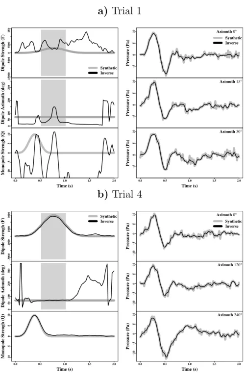
a)
Trial 1
Dipole Str engh (F) −15000 −5000 0 5000 15000 Synthetic InverseDipole Azimuth (deg)
0
50
100
200
300
0.0 0.5 1.0 1.5 2.0
−10 −5 0 5 10 Time (s) Monopole Str engh (Q) xx Pr essur e (P a) −5 0 5
10 Azimuth 0° Synthetic Inverse xx Pr essur e (P a) −5 0 5
10 Azimuth 15°
0.0 0.5 1.0 1.5 2.0
−5 0 5 10 Time (s) Pr essur e (P a)
Azimuth 30°
b)
Trial 4
Dipole Str engh (F) −3000 −1000 1000 3000 Synthetic Inverse
Dipole Azimuth (deg)
0
50
100
200
300
0.0 0.5 1.0 1.5 2.0
−10 −5 0 5 10 Time (s) Monopole Str engh (Q) xx Pr essur e (P a) −10 −5 0 5
10 Azimuth 0° Synthetic Inverse xx Pr essur e (P a) −10 −5 0 5
10 Azimuth 120°
0.0 0.5 1.0 1.5 2.0
−10 −5 0 5 10 Time (s) Pr essur e (P a)
Azimuth 240°
Trials 1 and 2. Trials 3 and 4 also show successful inversion, although their condition
numbers and standard deviations are significantly reduced. The result of fitting the
data and estimated source parameters from Trials 1 and 4 are compared in Fig. 2.3.
Even though both trials show good fits to the synthetic data, only the estimated
source parameters from Trial 4 are reliable. Therefore, in order to achieve stable
inversion, at least three stations covering 180◦ of azimuth are required. In Trials
5 and 6, the condition numbers are not reduced compared to Trial 4, though the
standard deviations decrease continuously. The experiment suggests that doing the
inversion at least 3 stations evenly distributed over 360◦ should produce the best
2.7
Infrasound radiation pattern and source
char-acteristics
2.7.1
Field experiment
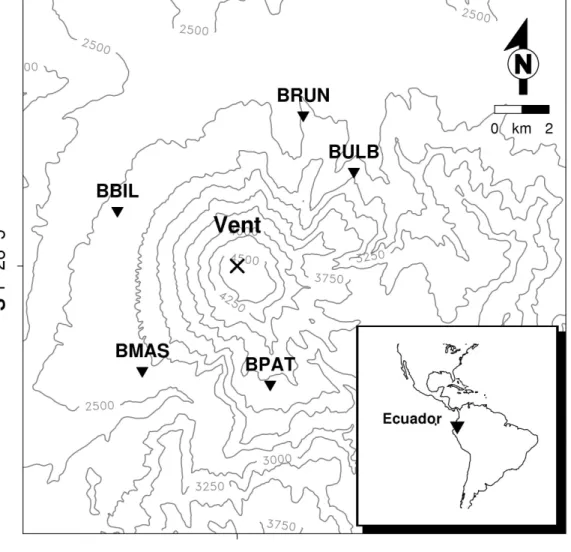
Tungurahua volcano is a large andesitic stratovolcano in the Cordillera Real of Ecuador.
The active vent, 5023-m high, is located on the upper part of its northwestern flank.
In May 2010, a new eruptive cycle began with a mid-size volcanic explosions
associ-ated with sustained ash column emissions, pyroclastic flows and seismic and infrasonic
tremor.
Between 2006 – 2010 a network of five broadband seismo-acoustic stations was
deployed by IGEPN (Instituto Geof´ısico – Escuela Polit´ecnica Nacional, Ecuador),
with support from Japan’s JICA program to monitor Tungurahua for hazard
mitiga-tion and volcano research. Each stamitiga-tion included an ACO Type-7144/4144 acoustic
sensor. The nominal infrasound sensor response was 0.1 to 100 Hz, with microphone
sensitivity 0.025 V/Pa and output voltage ±5 V. The amplifier-sensors were set to
record 893.5 Pa at full scale with sensitivity -0.005593 V/Pa, and a 100 Hz lowpass
filter was applied in the amplifier circuits. The microphones were designed specifically
to record in harsh volcanic settings. Distances between the vent and stations range
from 5.05 km at BPAT (Fig. 2.4) to 6.11 km at the furthest station BRUN.
Numerous infrasonic events were recorded during the period of May 28 – June 5.
Tungurahua infrasound records are characterized by short impulsive onsets
indicat-ing explosive eruptions. The peak magnitudes of these events were very large, up to
hundreds of Pa. The infrasound field recorded on the network exhibited clear
direc-tivity concerning radiation patterns: this strong direcdirec-tivity is not common in volcano
infrasound. In most cases, the highest amplitudes were observed at station BBIL
(Fig. 2.4). Although BPAT is the closest station from the active vent, recorded peak
cannot be explained by a simple monopole source. Accordingly, a model with a dipole
source may be required.
2.7.2
Inversion for source parameters
The multipole source model (monopole and dipole) was applied to the infrasound
records from Tungurahua, and the waveforms were inverted for source parameters.
Several assumptions were made: 1) We assumed that infrasound waves from
Tun-gurahua propagate into a half-space. Because of the slope (≈ 20◦) of Tungurahua,
infrasound spreads out over wider region than that of a hemispherical half-space. In
this case, inferred source strength from the half-space assumption is less than that of
the “true” source. 2) the acoustic wave intrinsic attenuation was ignored. Within the
lower atmosphere, the attenuation coefficient for frequencies ranging from 0.05 – 4
Hz is smaller than about 10−6dB/m which corresponds to a 0.1dB loss over a 100-km
path length (Sutherland and Bass, 2004; de Groot-Hedlin, 2008). Hence over the
5–10 km distance in our experiment, intrinsic attenuation is negligible. 3) Secondary
propagation effects such as reflection, refraction, and diffraction were not considered.
At short range and low elevation, the atmosphere is considered to be homogeneous.
Irregular topography was also ignored. BULB and BRUN were potentially affected
by reflection or refraction from local complex geometry. However, because there were
no barrier in the line between the vent and the stations and only short impulsive
events were chosen, the first single oscillation of signal is likely to be less affected by
reflection and refraction. 4) Wind effects are also ignored. Wind usually affects the
infrasound amplitude: a station in the upwind direction records larger amplitudes
than one in the downwind direction. Theoretically if the wind speed is Mach number
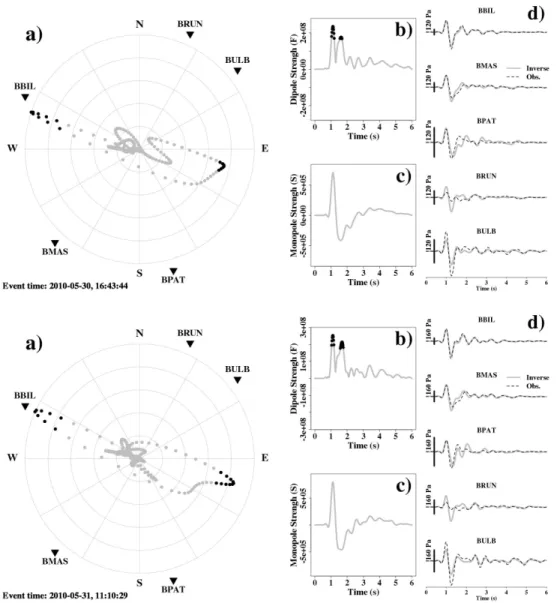
Table 2.2: Condition number and standard deviations of the source parameters for two events as shown in Fig. 2.5. S and |F| denote monopole and dipole strengths, respectively. Percentages of the standard deviation with respect to the estimates are given in parentheses.
Event time Condition No. S (kg/s) |F|(kg·m/s2) Azimuth (◦)
2010-5-30, 16:43:44 3.0×10⁵ ±2.9×10⁴ (4%) ±2.1×10⁷ (9%) ±3.2◦
2010-5-30, 17:45:03 3.0×10⁵ ±2.7×10⁴ (5%) ±2.0×10⁷ (9%) ±3.5◦
wind models of the Ecuadorean Civil Aviation Agency. With such low speeds, wind
effects on the sound amplitude are negligible. Since the peak amplitude ratio of BBIL
to BPAT in most cases exceeds 2 or 3, the amplitude difference is likely caused by
acoustic source characteristics rather than wind.
We selected 80 impulsive events during the period of the experiment, using only
data with high signal to noise ratio (40± 7 dB). The 6-s length signals were inverted
and source time functions for a monopole and dipole were simultaneously estimated
using Eq. (2.32). Integrating the source time function, the monopole strength S(t),
horizontal dipole strength F(t), and azimuth of the dipole axis were obtained (Fig.
2.5).
Because the amount of noise associated with the observations is unknown, it
is impossible to calculate exact variances of inverted model parameters using Eq.
(2.36). On the assumption of 10% noise with respect to maximum signal amplitude,
theoretical variances of the model parameters can be estimated (Table 2.2). These
variances do not represent “true” uncertainties underlying model estimates, but rather
provide insight on how stable model parameters with respect to data variability. Since
the signal-to-noise ratios for the selected events are high (≥ 33 dB), potential error
magnitudes associated with the events are not expected to exceed 10% of the signal
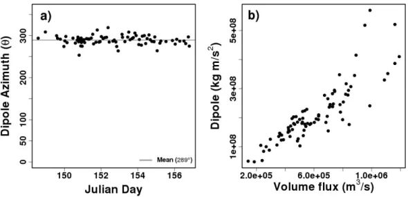
Figure 2.6: Estimated source parameters using events at Tungurahua volcano. a) Change of dipole azimuth during the field experiment. b) Volume flux estimated from monopole and dipole strengths.
2.7.3
Results
Two examples of the data fitting and estimated source parameters are provided in Fig.
2.5. In both cases the inversion results exhibit reasonably good fits to the data. The
largest misfits were associated with stations BRUN and BULB. While the observed
amplitudes from BRUN were consistently smaller than the fits, BULB showed larger
amplitudes than expected from the inversion. These two stations were located in areas
of complex terrain, with two wide and deep valleys nearby. Scattering and reflections
may be caused by the complex topography and terrain fluctuation. However, our
inversion procedure appears to be stable and the results are consistent (Fig. 2.5 and
2.6). We surmise that this is because we have used all the available stations for
inversion and site effects are not appreciable, leading to predicted pressures that are
close to observations.
b)
c) Source region
NW Effective Dipole
peak amplitudes. The low variances and associated condition numbers suggest that
the inversion procedure is stable.
The computed dipole vectors (Fig. 2.6a) show a consistent direction with mean
azimuth 289◦. The dipole direction was compared with the crater geometry of
Tun-gurahua. Tungurahua crater has a significant asymmetric shape (Fig. 2.7). The
north-west wall of the crater is 300 m lower than the south-east wall, and the
open-ing of the crater faces the north-west direction. The asymmetry of this feature was
confirmed by visual observation during the field campaign. Taking into account the
error of the DEM (produced by Instituto Geof´ısco Militar with 20 m resolution) and
the geometry changes involved with explosive eruptions, the opening direction and
the inferred dipole are considered to align significantly.
We also applied the simultaneous inversion method to “acoustic noise” that was
not related to volcanic eruptions in order to check the site effects such as an instrument
calibration and local noise. Noise data were chosen for different time periods over a
week, and the dipole direction was estimated (see the online supplementary materials).
Dipole directions from the noise were inconsistent with the 289◦ azimuth determined
from the volcanic source and indicated which stations showed the highest noise level at
that time. This suggests that the consistent dipole pattern observed from explosions
was not caused by site effects.
Volume flux associated with volcanic explosions can be calculated from the
esti-mated monopole strengths.
Q= 1
ρair
S(t), (2.37)
whereQ is volume flux,ρair = 1 kg·m3 is the air density, andS(t) is mass flux. The
dipole and monopole strengths for events at Tungurahua are well correlated (Fig.
During the experiment, it showed Vulcanian explosions with large ash columns and
large amount of ballistics (Ruiz et al., 2006; Fee et al., 2010). We compared the
volume flux with that of Augustine volcano, Alaska (Caplan-Auerbach et al., 2010).
The volume flux of Vulcanian eruptions of Augustine in 2006 were estimated using
infrasound observations to range between 2.6 – 6.2×10⁵m3/s. Because the vent radius
of Tungurahua (≈ 100m on May 2011) is larger than that of Augustine (≈30m), it
is reasonable that our estimated volume flux shows wider range, up to the order
of 106m3/s. We note that mass and volume outflux were estimated based on the
assumption of the constant standard atmospheric density in the vicinity of the vent.
If the vent is overpressurized or the volcanic jet significantly changes the composition
of air near the vent, the assumption will likely introduce significant errors in the
estimation. Even after taking the error of the density into consideration, however,
the volume flux remains comparable to the previous results. This suggests that our
multipole analysis is providing reasonable estimates of volume outflux during volcanic
explosions.
The magnitude of the dipole vectors was compared with those calculated from
observations at Mount Erebus, Antarctica (Johnson et al., 2008). The dipole vector
from bubble bursts at the Mount Erebus lava lake was estimated using an acoustic
dipole-solution in a free-space. The resultant dipole strength has a magnitude on
the order of 107 kg·m/s2. The acoustic signals used for the inversion showed peak
amplitudes of up to 200 Pa within a few hundred-meter distance from the source. Our
results indicate dipole vectors ranging up to 108 kg·m/s2. Although the Tungurahua
stations recorded 200 Pa peak at 5-km distance from the vent, the resulting dipole
strengths are comparable to those of Mount Erubus. Because the dipole strength
at Mount Erubus was calculated using a dipole-only model, the result may have
been over-estimated by incorporating part of the monopole into the dipole radiation,
strengths estimated for Tungurahua and Mount Erebus, although infrasound signals
at Tungurahua volcano show much stronger amplitudes.
It should be noted that modeling presented here only accounts for the horizontal
component of an arbitrary dipole in a half-space. The original dipole may include a
vertical component, but it cannot be estimated with the present station configuration,
as shown in Section 3. The real dipole may therefore be stronger than the estimated
horizontal results reported here.
Since monopole, dipole, and quadrupole source models of volcanic infrasound have
all been proposed (Woulff and McGetchin, 1976), it is still unclear which acoustic
source type dominates during volcanic explosions. A monopole source model was
used in studies of Strombolian explosions at Erebus and Karymsky (Lees et al., 2004;
Johnson et al., 2004, 2008), a large rockfall at Mount St. Helens (Moran et al., 2008),
and bubble oscillations at the lava surface at Shishaldin (Vergniolle and
Caplan-Auerbach, 2004), Stromboli (Vergniolle and Brandeis, 1994) , and Erta Ale (Bouche
et al., 2010). Only a few studies have addressed a dipole source model for volcanic
ex-plosions (Woulff and McGetchin, 1976; Vergniolle and Caplan-Auerbach, 2006;
John-son et al., 2008; Caplan-Auerbach et al., 2010). The acoustic network geometry may
be one reason for the lack of dipole modeling; full three dimensional radiation
pat-terns for a dipole solution are difficult to record on stations placed on the ground
surface.
2.8
Discussion
In general the source of volcanic infrasound is associated with atmospheric vibration
in the vicinity of the volcano vent. The acoustic source region is defined here by
distance, equations developed in Sec. 2 and 3 can be adapted for source inversion with
no modification. Once we consider the source as compact, there is an equivalence
be-tween the multipole solutions and physical pressure fluctuations in the source region,
similar to the force equivalence of a fault in seismology. In this section, we discuss
several possible source mechanisms inside the source region, which are attributed to
the inverted acoustic multipoles.
2.8.1
Direct Sources
Volcanic explosions and jets (or material flow) are direct sources of infrasound. Rapid
expansion of the compressed gas caused by explosions can be modeled as an acoustic
monopole, and represent the dominant source of the observed monopole. Moving
objects that subsequently exert forces on the fluid, however, contribute as a dipole
source. If the axis of the vent opening is inclined relative to the vertical axis, and
materials are ejected in this direction, the resultant effect will be equivalent to a
horizontal dipole component. Based on visual observation, the vent opening direction
at Tungurahua volcano was not significantly tilted from the vertical. In this case,
the vertical flow should be modeled as a vertical dipole, and the observed, strong,
horizontal dipole is not accounted for.
2.8.2
Diffraction and Reflection
The interaction of sound with solid boundaries inside the source region may account
for some of the observed radiation patterns. Theoretical calculations of sound
re-flection and diffraction using finite difference time domain (FDTD) method (Kim
and Lees, 2011) can be compared to multipole approximations. The southeast vent
wall at Tungurahua was represented by a semicircular, 200 m radial half disc, 200 m
computational domain, the three dimensional wavefield can be computed efficiently
in the cylindrical coordinate (Kim and Lees, 2011). A homogeneous medium (air
velocity = 340 m/s) was assumed and a monopole source of the gaussian function
(1 Hz corner frequency) was used to excite the sound field. A dipole source was not
used as the direct source because there is no evidence of significant horizontal fluid
flow discussed in Section 7.1., and vertical dipole does not contribute to the
hori-zontal asymmetric radiation. The frequency was estimated from observed infrasound
which showed peak frequencies near 1 Hz, rapidly attenuating at higher frequencies.
The source was placed on the disc axis by the wall illustrated in Fig. 2.8b. Sound
pressures were obtained on the half-space boundary, 3 km distant from the source in
all azimuthal directions, well enough away such that near-field effects can be ignored.
Amplitudes, relative to the maximum amplitude in the propagating sound field, were
then assumed to be measures of the effects of reflection and diffraction.
The modeled pressure distribution, compared with the multipole radiation pattern
determined by observations, is shown in Fig. 2.9. The peak-amplitude ratios of each
station relative to BBIL station are presented showing a considerable variance. The
large variance is probably attributed to either complex source mechanisms which
cannot be explained by the combination of the monopole and the dipole or to local
noise at the stations. Because the amplitudes are ratios of each station to BBIL,
local noise at BBIL has a compounding effect on variance in this plot. Even though
the observed amplitudes show such a large variance, the inversion method appears to
point to the best-fit solutions including a monopole and dipole.
While the monopole produces an omni-directional radiation, the dipole contributes
to the varying amplitude dependent on the azimuthal direction. The dipole produces
a positive amplitude of the first arrival in BBIL direction, which constructively
This destructive interference with the positive monopole produces a small, positive
amplitude at BPAT. Because the observed dipole is alternating (Fig. 2.5a), the dipole
direction is reversed after the first arrival, giving a large negative amplitude at BBIL
and small negative amplitude at BPAT (Fig. 2.5d) due to interference with the
neg-ative monopole (Fig. 2.5c). Even though the strength of the dipole is larger than
the monopole by an order of ∼102 (Fig. 2.6), the combined radiation pattern shows
positive amplitudes of the first arrival at all five stations. Because a dipole is
rep-resented by two alternating, closely spaced, monopole sources, the radiated energy
cancels, and is a much less efficient source than a monopole source (Lighthill, 1952).
The diffraction (and reflection) shows the characteristic directional pattern
pre-sented in Fig. 2.9. The smallest radiation amplitude does not occur immediately
behind the wall, but rather appears slightly off that direction. This is because
edge-waves diffracted at the edge of the disc are superposed constructively at the axis of
the disc, and destructive interference occurs slightly off the axis. In comparison with
the multipoles, the directivity of the diffraction is remarkably aligned with it. The
diffraction pattern explains well the large amplitude at BBIL and the small
ampli-tude at BBAT. However, it is evident that the degree of directivity of the multipole
is larger than expected from the theoretical diffraction pattern. The observed ratio
of BPAT to BBIL (median value ' 0.15) is smaller than the value of 0.4 expected
from the diffraction alone, suggesting that the amplitude of BBIL is much larger.
This discrepancy is too large to be explained by modeling errors associated with the
simplified model. Of course, assumptions of a semicircular back-wall and inaccurate
wall dimensions may give rise to errors in the obtained diffraction pattern. At low
frequency (1 Hz peak frequency, wavelength = 340 m), however, variations in wall
dimensions of up to several tens of meters will not affect the diffraction radiation
patterns significantly. This suggests that the diffraction effects partially influenced