1
THE TRANSITION TO LOW FERTILITY IN BRAZIL
Raquel Zanatta Coutinho
A dissertation submitted to the faculty at the University of North Carolina at Chapel Hill in partial fulfillment of the requirements for the degree of Doctor of Philosophy in the Sociology
Department Program in the College of Arts and Sciences
Chapel Hill 2016
Approved by: S. Philip Morgan Lisa D. Pearce Yong Cai
ii © 2016
iii
ABSTRACT
Raquel Zanatta Coutinho: The Transition to Low Fertility in Brazil (Under the direction of S. Philip Morgan)
iv
v
To my parents, Maria Teresa and Marcelo, My most cheerful supporters.
To my second mother Cecilia (in memoriam), I hope you accept this PhD as yours.
To my husband, Andre, My encouragement and inspiration.
To my son, Theodor,
vi
ACKNOWLEDGEMENTS
Writing a dissertation wasn’t easy, but wasn’t lonely. Getting here was a collective effort. I have tons of people I have to thank for helping me get through these 5 years of the PhD
program. Below, I list only some of the wonderful people I had the pleasure to meet. I apologize if my memory fails me now.
I would like to first thank my advisor, Professor Philip Morgan, for believing this was possible. Thank you for understanding my priorities, for supporting me in my decisions, and for the excellent mentoring you gave me in the last years. I will need to write many papers, teach many classes and advise many students so that I can use all the knowledge you have passed to me. Thank you!
I thank Professor Lisa Pearce for being my advisor in the first half of this program, but also for continuing to collaborate and enrich my formation. Thank you for your patience, for serving as a guide, and for teaching me the highest standards of mixed-methods research.
Professor Catherine Zimmer, thank you for being such an important source of security in the middle of this thunderstorm. Your enthusiasm, concern for the students and passion for statistics are unbeatable.
vii
Professor Joseph E. Potter (University of Texas at Austin), thank you for inviting me to work on the BCAS project in 2007 when I was just an undergraduate student, because that is where my passion for sociology began. I have learned a lot from you over the years and it is an honor to have you on my PhD committee.
In sum, for all of my committee members, thank you for the wonderful contributions to my dissertation. I admire your work very much and it is marvelous to see your personalities shining on my papers.
I also thank all my other professors here at UNC. It has been fabulous to learn so much from you: Howard Aldrich, Andy Andrews, Neal Caren, Guang Guo, Kathie Harris, Arne Kalleberg, Charles Kurzman, Laura Lopez-Sanders, Ted Mouw, Andy Perrin, Mike Shanahan, and Claire Yang. I hope I can reproduce your high standards wherever I go.
I also thank the staff members for all their help: Sandy Wilcox, Kelsea McLain, Mary Chyatte, Karen Judge, Pamela Stokes, Jimena Loyola, Reggie Singletary, Ben Haven. I thank Gigi Taylor, from the Writing Center, for caring so much for the international students and Jan Hendrickson-Smith and her husband Doug Hendrickson-Smith, for taking care of me.
I will be forever thankful to the Department of Sociology at University of North Carolina at Chapel Hill for opening their doors to me, funding my graduate course and transforming my career. Thanks for considering my application and taking my dreams seriously.
viii
I also thank the wonderful Brazilians who helped to make my stay warm and fun: Vanessa Veiga, Thiago Nicolini, Rodolfo Coppo, Kassio Zanoni, Priscilla Ferreira, Rosangela Pereira, among so many others. You became my home away from home and I hope we can continue to be friends once we are all back to our country.
Alisson Barbieri, my mentor from Brazil, UNC alumni: thank you for the support bringing me to UNC, for the career related advice during these 5 years and thank you for doing your best to make sure our country can take advantage of what I learned here.
Shakti, Manoj and Ayush Tripathy, thank you for taking care of Theodor as your own son. Outsourcing my motherhood from 9 AM to 5 PM wasn’t very fun, but I am really blessed for having you do the most precious job in the world. I could not have someone better!
I also thank all the graduate students I met on my way. In particular, Sarah Gaby, Kari
Kozlowski, Sally Morris, Carmen Bapat, Jordan Radke, Jessica Pearlman (especial thank you for your statistics advices), Ali Kadivar , Charles Seguin, David Rigby, Jason Freeman, Joseph Crane, Batool Zaidi, Laura Krull, Anna Rybinska, Atiya Hussain, Luke Sherry, Jane Lee, Anne Hunter, Emily Mckendry-Smith, Tiantian Yang, Ricardo Martinez, Shradha Shrestha, Karam Hwang, Autumn McClellan, Joseph Bongiovi, Shane Elliot, Jessica Zhenhua Xu, Tim Cupery, Brian Levy, Ashton Verdery, Jonathan Horowitz, Aniket Bera, and many others. Thank you for your friendship. I will miss these years, this town, this group of amazing folks who certainly made the work more enjoyable than one expects from a PhD program. I will always cheer for your success.
ix
also thank the Demography Department (Cedeplar/UFMG/Brazil) for making me a visitor scholar during my Leave of Absence in 2014/2015, so I could have office space.
With all my love, I thank my wonderful cohort members, Brian Foster, Courtney Boen, Daniel Auguste, Didem Turkoglu, Haj Yazdiha, Holly Straut, Karen Gerken, Kristen Schorpp, and Michael Good (as well as their wonderful significant others Dan, Josh, George, Travis, Sarah, Alyssa and Luna). I cannot mention enough how wonderful you have been to me and how forever thankful I will be for everything you did to me. I love you very much and I hope you all become rich and famous, so you can come to Brazil very often.
The friends I left in Brazil: Angela Azevedo, Marcia Romano, Jamila Alvarenga, Marina Mattos, Sofia Lopes, Gabriela Bonifacio, Helena Castanheira, Ana Paula Verona, Maria Carolina Tomas, Vanessa Di Lego, Terezinha Assumpção, Nice Farias, Carlos Gohn, Nelci Muller, Maria Ignez Moreira, Solange Mattos, Zilda Machado, Leoncio Soares, Geruza Souza, Fernanda Neri and Jania Pereira. Thank you for being my friends even though I kept moving abroad. For the older folks: thank you for taking care of my parents while I was away.
To my wonderful family. My grandparents Maria and Jose Zanatta (both in memoriam), and Maria Celia and Vinicius Coutinho, thanks for being such a great example of family life and affectionate love. Thank you for putting together such a big and beautiful family.
x
thanks for teaching me about how cool a DINC couple can be. And thank you for moving so close to mom and dad, so your sister can be more adventurous knowing they are in good hands.
My marvelous aunt Maria Cecilia Zanatta, the biggest hearted being I have ever met, but who left this world in the same month she got accepted into a PhD program in Psychology, after a short and unfair battle against cancer in 2015. The news about your PhD acceptance brought you so much hope and light in the middle of that chaos. I know this was your dream and I know how happy you were for me and how supportive and cheerful you have been in every single process of the way. Thank you for everything! Wherever you are, I know you are doing your research and I know you continue to look over us. I love you and miss you incredibly.
xi
My son, Theodor, thank you for bringing me back to my priorities and for making me re-think every single theory of fertility I learned in the last years. No one has taught me more about motherhood than you.
I also thank the universe for allowing me to be here today. When I came to Chapel Hill in August 2011, I still had stiches from an abdominal surgery and was forbidden by the doctors to carry my own bags. I have been 5 years cancer free and now I have a son, a PhD, wonderful memories to share and a brand new chapter waiting to be written. I hope I can continue to do social sciences for a living and I hope I can help make the world a better place for my son’s generation and beyond.
O correr da vida embrulha tudo. A vida é assim: esquenta e esfria, aperta e daí afrouxa, sossega e depois desinquieta. O que ela quer da gente é coragem.
xii
TABLE OF CONTENTS
LIST OF TABLES ... xv
LIST OF FIGURES ... xviii
LIST OF ABBREVIATIONS ... xx
CONTEXTUALIZING THE BRAZILIAN FERTILITY TRANSITION ... 1
Importance ... 4
Theoretical and Methodological Frameworks ... 5
The Theory of Conjuntural Action ... 5
The Bongaarts Proximate Determinants of Fertility ... 7
CHAPTER 1: AN APPLICATION OF THE BONGAARTS PROXIMATE DETERMINANTS OF FERTILITY FOR BRAZIL ... 9
INTRODUCTION ... 9
METHODOLOGICAL AND THEORETICAL FRAMEWORKS... 12
CONCEPTUALIZATION, DATA AND MEASUREMENTS ... 18
Covariates ... 30
Data ... 31
RESULTS AND DISCUSSION ... 32
General model ... 32
Parameters ... 33
1 -Total fertility rates in Brazil ... 34
2 - Desired family size ... 35
xiii
4 - Child replacement ... 39
5 - Sex preferences ... 40
6 – Tempo Effect ... 41
7 - Infecundity and Involuntary Childlessness... 42
8 - Competing preferences ... 43
CONCLUSION ... 45
CHAPTER 2: SEX PREFERENCES IN BRAZIL ... 56
INTRODUCTION ... 56
LITERATURE REVIEW ... 59
Mechanisms and explanations for sex preferences ... 59
Empirical evidence and hypotheses ... 63
DATA, LIMITATIONS AND EX POST-RATIONALIZATION ... 70
VARIABLES, METHODS AND RESULTS ... 76
Descriptive analysis ... 78
Desired Sex Ratios ... 79
Multinomial Logit Regressions... 81
DISCUSSION ... 90
CHAPTER 3: SHEDDING LIGHT ON COMPETING PREFERENCES ... 106
INTRODUCTION ... 106
What competes with motherhood?... 111
Education ... 112
Work/Career ... 116
Lack of partner ... 119
Late transitions ... 120
xiv
First objective... 123
Second objective ... 127
Third objective ... 132
Fourth objective ... 135
DISCUSSION ... 140
APPENDIX 1: CHAPTER 1 ... 164
APPENDIX 1.2: CHAPTER 1 ... 169
APPENDIX 2: CHAPTER 2 ... 171
Does intention translate into behavior?... 180
APPENDIX 3: CHAPTER 3 ... 188
xv
LIST OF TABLES
Table
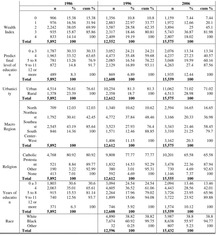
1.1. Characteristics of the Brazilian DHS 1986 and 1996 and PNDS 2006
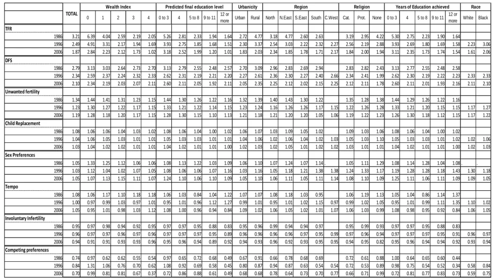
samples utilized in this chapter……….. 48 1.2. Values for the parameters of the Bongaarts Proximate Determinants of
Fertility calculated with the Brazilian DHS 1986 and 1996 and PNDS
2006………. 49
2.1. Actual composition by ideal composition for women who only want one child, Brazil, 2006 and 1996………... 94 2.2. Actual composition by ideal composition for women who want two
children, Brazil, 2006 and 1996………. 95 2.3. Actual composition by ideal composition for women who want three
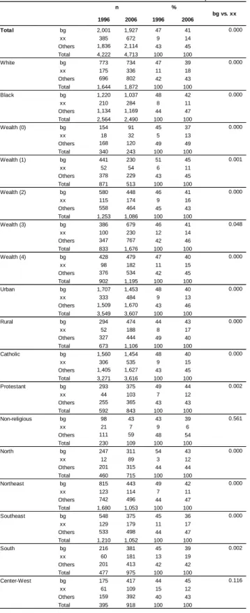
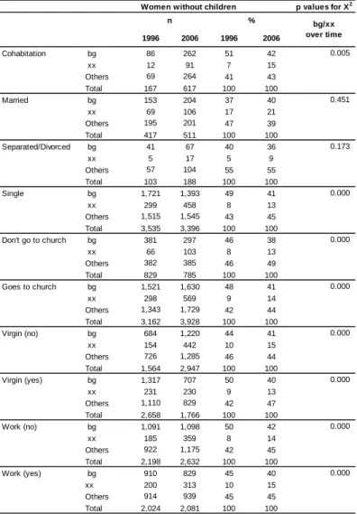
children, Brazil, 2006 and 1996………. 96 2.4. Decline is the proportion of women who report bg (balance) as ideal
composition and increase in the proportion who report xx (indifference) as ideal, all women without children, Brazil, 1996 and 2006………. 97 2.5. Total Desired Sex Ratios of women without children and of women with
children, Brazil, 1996 and 2006………. 99 2.6. Desired composition sample distributions by desired parity, women
without children, Brazil, 1996 (n=3935)………. 100 2.7. Desired composition sample distributions by desired parity, women
without children, Brazil, 2006 (n=4263)………. 101 2.8. Multinomial logistic regression of desired composition, women without
children, Brazil, 1996 and 2006………. 102 2.9. Multinomial logistic regression of desired composition, women without
children who want one child, Brazil, 1996 and 2006……… 103 2.10. Multinomial logistic regression of desired composition, women without
children who want two children, Brazil, 1996 and 2006………. 104 2.11. Logistic regression of desired composition, women without children who
xvi
3.1. Univariate and Multivariate Poisson regressions of Children Ever Born,
women age 40 and plus, Brazil, 1986, 1996 and 2006……… 155 3.2. Univariate and Multivariate Poisson of Desired Family Size, all women,
Brazil, 1986, 1996 and 2006……….. 155 3.3. Multinomial logit of Fertility Status, all women aged 30 and plus, Brazil,
1986, 1996 and 2006. Reference category is Surplus……… 156 3.4. Logit regressions of Not wishing to have more children (reference=1)
compared to people who wish to have it later (0), women who have
CEB<DFS, women age 30 and plus. Brazil, 1986, 1996 and 2006……… 156 3.5. Total count of children who were born in excess (if DFS-CEB <0,
Surplus), who were not born (if DFS-CEB>0, Deficit) and born according to their mother's CFS (DFS-CEB=0, Neutral), all women, Brazil, 1986, 1996 and 2006………...
157
3.6. Estimates of Deficit Fertility based on women's report for Ideal Family Size compared to estimates of Competing Preferences (FC) measured as
a residual of the Bongaarts equation and compared to the multiplication of the Competing Preference residual (FC) by Tempo effect (FT)and
involuntary infertility (FI), values for Brazil, 1986, 1996 and 2006…….. 160
3.7. Estimates of Surplus fertility based on women's report for Ideal Family Size compared to estimates of Unwanted fertility (Fu) measured as the Bongaarts equation and compared to the Unwanted (Fu) multiplied by sex preferences (FSP)and child replacement (FR), values and Pearson
correlations for Brazil, 1986, 1996 and 2006………...
161
3.8. Desired Family Size by survey year, age groups and selected covariates,
Brazil………. 162
3.9. Measures of dispersion for Desired Family Size by survey year, age
groups, birth cohort and number of children ever born in 1986, Brazil…. 163 A2.1. Top 5 preferred composition, women without children, Brazil, 1996 and
2006……… 171
A2.2. Proportion of women who desires additional children given her current composition and probabilities that the proportions are the same, women
with only one child, Brazil, 1996 and 2006……… 176 A2.3. Proportion of women who desires additional children given her current
composition and probabilities that the proportions are the same, women
xvii
A2.4. Parity Progression Rates by selected variables, all women with children Brazil,
1996……… 178
A2.5. Parity Progression Rates by selected variables, all women with children
Brazil, 2006………. 179 A3.1. Population values for: mean years of education, mean age at first union
and proportion of women in the labor force by survey year. Brazil, DHS
1986 and 2996 and PNDS 2006………. 188 A3.2. Calculation process of Adjusted Deficit and Adjusted Surplus
xviii
LIST OF FIGURES
Figure
1.1. Parity progression ratios by parity. Brazil, 2006. Borrowed from
Bonifacio (2011 p. 18)………... 50
1.2. Difference between Total Fertility Rates and Desired Family Size in number of children……… 50
1.3. Parameter for Unwanted Fertility, Brazil, 1986, 1996 and 2006……….. 51
1.4. Parameter for Child Replacement, 1986, 1996 and 2006………. 51
1.5. Parameter for Sex preferences, 1986, 1996 and 2006………... 52
1.6. Parameter for Tempo, 1986, 1996 and 2006………. 52
1.7. Parameter for Involuntary Infertility, 1986, 1996 and 2006……….. 53
1.8. Parameter for Competing Preferences, 1986, 1996 and 2006…………... 53
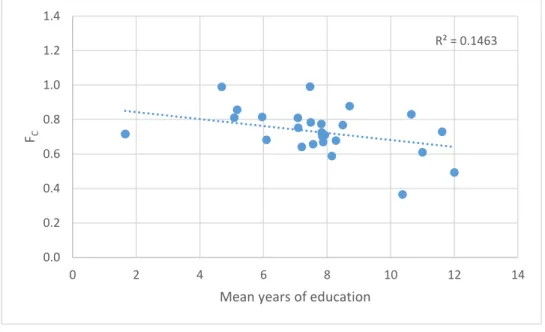
1.9. Scatterplot of the Competing Preferences values with the population mean values for years of education, Brazil (1986, 1996, 2006), all socio-demographic groups………. 54
1.10. Scatterplot of the Competing Preferences values with the population mean values for years of education, all socio-demographic groups, Brazil, 1986……… 54
1.11. Scatterplot of the Competing Preferences values with the population mean values for years of education, all socio-demographic groups, Brazil, 1996……… 55
1.12. Scatterplot of the Competing Preferences values with the population mean values for years of education, Brazil, 2006……….. 55
2.1. FC by mean age at first union, Brazil, 1986………... 150
2.1. FC by mean age at first union, Brazil, 1996………... 150
2.3. FC by Mean age at first union, Brazil, 2006………... 151
2.4. FC by proportion of women working, Brazil, 1986………... 151
xix
2.6. FC by proportion women working, Brazil, 2006……… 152
2.7. Correlation between Deficit and (FC), Brazil, 2006………... 153
2.8. Correlation between Deficit and (FC)*(Ft)*(Fi), Brazil, 2006…………... 153
2.9. Correlation between Deficit and (FC), Brazil, 1996……….. 153
2.10. Correlation between Deficit and (FC)*(Ft)*(Fi), Brazil, 1996…………... 153
2.11. Correlation between Deficit and (FC), Brazil, 1986……….. 153
2.12. Correlation between Deficit and (FC)*(Ft)*(Fi), Brazil, 1986…………... 153
2.13. Correlation between Surplus and (Fu ), Brazil, 2006………. 154
2.14. Correlation between Surplus and (Fu )*(Fsp)*(FR), Brazil, 2006……….. 154
2.15. Correlation between Surplus and (Fu ), Brazil, 1996………. 154
2.16. Correlation between Surplus and (Fu )* (FSP)*(FR), Brazil, 1996………. 154
2.17. Correlation between Surplus and (Fu ), Brazil, 1986………. 154
xx
LIST OF ABBREVIATIONS
ASE Asymptotic Standard Error BA Bachelor Degree
BEMFAM Sociedade Civil Bem-Estar Familiar no Brasil CDD Center for Disease Control
CEB Children Ever Born
CEBRAP Brazilian Center for Analysis and Planning CNJ Conselho Nacional de Justica
DFC Desired Family Composition DFS Desired Family Size
DHS Demographic and Health Survey DSR Desired Sex Ratios (DSR)
EPSEM Equal probability of selection method FC Competing preferences
FI Involuntary infertility
FR Replacements for child mortality
FSP Sex preference
FT Tempo effect
FU Unwanted fertility
IBGE Instituto Brasileiro de Geografia e Estatística LA Latin America
xxi
PNAD Pesquisa Nacional por Amostra de Domicílios PNDS Pesquisa Nacional de Demografia e Saude PPS Probability proportion to size
PSM Propensity Score Matching RRI Relative Risk Ratio
SDT Second Demographic Transition SRLB Sex Ratio at Last Birth
TCA Theory of Conjunctural Action TFR Total Fertility Rate
TV Television
UNESCO United Nations Educational, Scientific and Cultural Organization UNICEF United Nations Children's Fund
1
CONTEXTUALIZING THE BRAZILIAN FERTILITY TRANSITION
Until recently, policymakers in developing countries were concerned about the contribution of high fertility rates to rapid population growth and to poor urban and
socioeconomic conditions (Bongaarts, 2001). Today, low fertility is a widespread phenomenon. More than half of the world’s population lives in a country where fertility is below replacement level (Morgan, 2003; Morgan and Taylor, 2006). Brazil is now one of them (Potter,
Schmertmann, Cavenaghi, 2002; Carvalho and Brito, 2005; Potter et al. 2010). Total Fertility Rates went down from 5.8 children per women in 1960 to 1.91 in 2010 (Brasil, 2010). This decline in fertility represents a cultural change without any foreseeable return, instigating the convergence of all social groups to smaller family sizes (Carvalho, 1998)1.
Aside from distal factors such as economic development, modernization,
industrialization, urbanization, mass education, rural exodus, and increased participation of women in the labor market, researchers attribute the primary proximate determinant of the decline in fertility to an increased usage of contraceptive methods, especially female sterilization (Curtis and Diamond, 1995, Potter, 1999; Potter, Schmertmann, and Cavenaghi 2002).
Sterilization helped women restrict fertility at higher orders (Bongaarts, 1999) and caused a rejuvenation in fertility rates, which would be even more important for women without high
2
school education (Alves and Cavenaghi, 2009). That, on top of the relative increase in the
participation of low order births for the fertility rates caused a negative tempo effect inflating the Brazilian TFR (Miranda-Ribeiro, Rios-Neto and Carvalho, 2013).
Researchers found that 75% of women engaged in a conjugal union before age 24; and 75% of women who were sterilized did so before age 25. As a result, a significant percentage of women gave birth to all their children by age 30 (Miranda-Ribeiro, Rios-Neto and Carvalho, 2013), a very early start that seemed nothing like the profiles observed in Europe (Alves and Cavenaghi, 2009). As Bonifacio (2011) points out, what makes Brazil unique is that it was possible to achieve low fertility even with adolescent childbearing and an early age at marriage.
But a different phenomenon began to take place: the birth control pill gained traction as a method of contraception, and women no longer had to rely on irreversible methods to control their fertility, allowing women to wait longer to start having children and to space the births over time. They were also no longer tied to the obligation to have a minimum number of children before accessing contraception (Caetano and Potter, 2004).
Surprisingly, around the year 2010, researchers started to notice changes to Brazilian fertility rates. First, a reduction in teenage fertility rates was observed (Silva and Surita, 2012). Second, the tempo effect got closer to zero suggesting the stabilization of the mean age at childbearing (Miranda-Ribeiro, Rios-Neto and Carvalho, 2013). A small postponement of fertility for upper class and high educated women was also recorded. The mean age at
3
2009).2 The percentage of women having children by age 30 has been consistently decreasing ever since (Rosero-Bixby, Castro-Martín, Martín-García, 2009).
In Brazil, important differences persist regardless of the low value at the aggregate level. The total fertility rate in 2006 in Brazil reached 1.8, below replacement level, and fell to 1.1 for women with at least 12 years of education (Ministério da Saúde,2008). Those with 0 to 3 years of education still had a TFR of 3.14 children but with downward trends3. This polarized behavior is also a reflection of the high levels of inequality, despite the recent improvements. Brazilian HDI has shifted from 0.557 in 1985 to 0.633 in 1995 and to 0.699 in 2005. The most recent is of 0.730 in 2012 (UNDP, 2013).
Variations by region, income level and race/ethnicity have also been reported in recent years. White women had a TFR of nearly half a child less than blacks (TFT=1.53 for whites and 1.98 for blacks) in the year 2006. For the same year, women with a per capita income equal to 1/4 of the Brazilian minimum wage had a TFR of 4.8 in 2006, while women with a per capita income equal to the minimum wage had a fertility rate below replacement starting in the early 2000´s (Berquó and Cavenaghi, 2006). Other variations, such as regional disparities, are also pronounced. For example, inhabitants of the north region had a TFR of 2.28 while those of the south had a TFR of 1.69. Even controlling for socio-economic status, research indicates that regional differentials exist (Alves and Cavenaghi, 2009). The most recent census in the year
2 Alves and Cavenaghi utilized a more recent dataset (Census and PNAD) when compared to Bonifacio (2011), who used the same data I am using, the Brazilian PNDS.
4
2010 confirms that regional differences are still remarkable, although the gaps have been narrowing (Miranda-Ribeiro and Garcia, 2012)4.
Importance
That gaps between socio-demographic groups have been narrowing suggests that at the level of intention, fertility might not be as varied among social groups as outcomes are. It is possible that the degree of preference implementation is what has now been keeping women at different rates. While much descriptive analysis has explored fertility variation, other than unwanted fertility and tempo effect, little attention has been paid to what drives fertility differentials in Brazil and the mechanisms of these social influences. Thus, it is still unclear whether in Brazil younger cohorts seems to be having different aspirations and behaviors regarding marriage, family and career or if they are facing obstacles to achieving their desires.
By exploring fertility variation and its components across time in Brazil, this paper illuminates the factors that contribute to low fertility, how these factors combine to form the total fertility rate throughout the years and how they vary by socio-demographic characteristics (race, religion, education, geographic macro-region, and place of residence). This series of papers answer some questions that have remained open in the recent literature exploring the same topic (Bonifacio, 2011; Carvalho, 2014). Some of these questions pertain to socio-demographic differences in fertility (Paper 1), such as what makes less educated and rural women bear more children - do they still have higher fertility ideals or are there other factors influencing their
5
fertility rates? Other questions relate to the degree of preference implementation when women are faced with mediators between her desired family size and her actual behavior (Papers 2 and 3). The two factors that will be explored in depth in this work are gender preferences (i.e. the desired sex composition of your children) and competing preferences for motherhood (i.e. other life choices that compete with childbearing causing women to review her desired intentions downwards, such as prolonged education, career and lack of partner5).
In the following paragraphs, I will briefly introduce the Theory of Conjunctural Action and the Bongaarts Proximate Determinants of Fertility, which are respectively the theoretical and methodological frameworks I use to explore the determinants of low fertility in Brazil.
Theoretical and Methodological Frameworks
The Theory of Conjuntural Action
From a sociological perspective, the number of children a women will have during her lifetime is shaped by societal influences, but is also influenced by the individuality of
biographies and the resources, or materials, through which women could successfully achieve their ideals. The Theory of Conjunctural Action (TCA) (Johnson-Hanks et al. 2011) explains this interplay. The mechanism through which the influences operate is defined as schemas, the expected ideas and behavior one learns by induction or direct exposure overtime through socialization and interaction. Characteristics such as religious affiliation or place of residency provide women with different ideal family sizes and compositions.
6
In Brazil, the ideal number of children seems to be contingent upon structural influences. For example, women in rural areas have higher desired family sizes when compared to urban women. In terms of gender preferences, schemas also help couples make reproductive decisions, for example, in rural areas sons are more useful than daughters, and so a couple might decide to continue childbearing until a son is born.
But since fertility has been going down and differences in population subgroups
narrowing, there are reasons to believe that the desired family sizes and compositions are more similar among all segments of society, demonstrating either a weakening of societal norms or a convergence of schemas toward low fertility targets or replacement level. Nonetheless, the number of children ever born, or the total fertility rates, continue to be different among the various segments, suggesting that materials resources (e.g. resources), such as access and implementation of contraceptive methods, could have been more important in defining fertility than the social structures that govern this ideals. This explains, for example, how women with higher income have much smaller unwanted pregnancy rates, although they might have desired family sizes that are similar to their less educated counterparts’.
But the differences cannot be attributed solely to a variation in materials or schemas. The life course is embedded in a social context which brings about conjunctures that might affect existing plans and make, for example, women take different decisions than expected. While unemployment might delay fertility for some, it might be just the right excuse to start having children for others. “Demographic models of family change and variation have tended to assume
7
what women imagine as an ideal number of children and how many children she ends up having can vary. It is their experiences prior, during and after each birth that will shape the final number of children ever born (Morgan and Taylor, 2006).
For instance, a qualitative study of Brazilian women identified several situations in which life didn’t go as planned (Carvalho, 2014). In Carvalho’s sample, while some women took longer than expected to get married, others ended up with unwanted pregnancies. In both cases, fertility didn’t go as women had anticipated. Carvalho (2014) also finds, for example, that women changed their minds about the ideal number of children or ideal sex composition after having their first child or after getting married.
The Bongaarts Proximate Determinants of Fertility
Many theoretical and methodological models are available for researchers of low fertility (Morgan and Taylor, 2006). In 2001, Bongaarts6 described a theoretical model that aimed at explaining fertility rates at the aggregate level (TFR) as a result of the multiplication of six parameters by the Desired Family Size (DFS). The first group of parameters is composed of factors that enhances fertility related to desired family size: unwanted fertility (FU), replacements for child mortality (FR), and sex preference (FSP). The second group is composed of factors that
decrease fertility related to desired family size: rising age at childbearing (tempo effect which would be the number of children that a women would have had if they had not waited, or the FT), involuntary infertility (which includes the inability to have a child and also an inability to find a
8
suitable partner, the FI), and competing preferences for child (set to 1 when childbearing is
universal, the FC). Thus,
TFR = DFS * (FU * FR * FSP) * (FT * FI * FC)
If woman realizes her fertility intention, TFR=DFS.
Different values for each parameter is what causes women that have the same fertility ideals to end up with different fertility outcomes. By exploring fertility variation and the
different values for the above components across time it is possible to understand what has been driving fertility decline and how different socio-demographic characteristics (age, race, marital status, religion, education, geographic macro-region, and place of residence) behave in the presence of the same factors. Using decompositions and proximate determinant models has been proved to be a valuable tool to aide conceptualization, explore variations, revise theories and of course, produce what Morgan and Taylor (2006) call “what we know”, or what all scientists can agree on regardless of their theoretical stand point.
9
CHAPTER 1: AN APPLICATION OF THE BONGAARTS PROXIMATE DETERMINANTS OF FERTILITY FOR BRAZIL
INTRODUCTION
10
2010, confirms that these persist, although the gaps have been narrowing (Miranda-Ribeiro and Garcia, 2012)7.
Determining the causes and consequences of the fertility transition and the fertility decline below replacement has kept many generations of demographers busy (Mason, 1997). Nevertheless, it is for a good reason. Scholars need to know variations in desired fertility but also how often people are able to implement their fertility preference and the reasons why observed fertility departs from desired family size. In contemporary developed countries it is common to find that desired family size is higher than total fertility rates (Bongaarts, 2001). Besides, the unwanted long term consequences of fertility below replacement, such as population aging and decreasing rates of growth that turn negative with time, could be problematic in some countries. European and some Asian countries, for example, start to feel the first signs of an unbalanced age structure. Lutz et al (2003) demonstrate that the effects so far have been small in Europe, but each additional decade that fertility remains below replacement represents a decline from 25 to 40 million people (in the absence of immigration or changes in current mortality rates).
Much of the decline might actually be an effect of postponement of fertility, as argued by Bongaarts and Feeney (1998), the so called “tempo effect”. If this is true, one might see reversals in fertility rates in the future, when women stop further postponement (Morgan, 2003). However, some of these women might not have time (or the desire) to “recuperate” postponed fertility and others might decide to never have children at all. Thus postponement can generate a “quantum effect” (Caldwell and McDonald, 2006; Lesthaeghe and Willems, 1999). In fact, research shows that changes do not seem to be only a timing effect, but a reduction in the number of births,
11
which can have severe implications for the “lowest-low” fertility countries (Myrskyla et al. 2012).
Different from trends observed in Europe, Brazilian fertility remains early (Rios-Neto et al. 2005; Alves and Cavenaghi, 2009). In fact, Brazilian research suggests that any ‘tempo effect” might have been negative – a shift to younger ages at birth may have depressed the observed TFR (Miranda-Ribeiro et al. 2006). According to the authors, the mean age of childbearing that was 29.5 in 1970 dropped to 26.5 in 1994. Part of this decline is due to a decline in higher parity births as can be seen in Table 1.1 (borrowed from Bonifacio, 2011). That means the mean age at childbearing would be higher if women were continuing to have children throughout her reproductive life.
More than half of all women in the 20-25 age group were already mothers in 2006 (BEMFAM, 1987 and 1997; Ministerio da Saude, 2008). The same data shows that 25% of the women who got sterilized, did so before the age of 25, putting an end to their reproductive period at ages before women in Europe were having their first child. The only signs of postponement in Brazil are found among women of higher education levels8 (Ministerio da Saude, 2008).
The mean age of childbearing has increased modestly in the last decade (Miranda-Ribeiro and Garcia, 2012). Drawing on Lesthaegue and Willems (1999) and after observing
postponements for the second child, Miranda-Ribeiro and Garcia (2012) suggest that Brazil is entering the second phase of the demographic transition, where after fertility levels decline for all ages and parities, women start postponing fertility. The authors also suggest that there is an
12
unexplored variation in fertility that should be understood if one wishes to predict Brazil’s future fertility.
Factors associated with fertility decline could be different for each country, and the speed of the decline tied to each country’s internal disparities. The substantial differences in the
European transition makes studying low fertility in Brazil an opportunity to understand how interactions and changes in social institutions and in preferences shape Brazil’s fertility. Thus, this chapter explores fertility variation and its components across time in Brazil, shedding light on the factors that contribute to low fertility, how they vary by socio-demographic characteristics (race, religion, education, wealth, geographic macro-region, and place of residence), and how these factors combine to produce the total fertility rate and its variation across groups and time period. My work uses the Demographic and Health Survey data from 1986, 1996 and 2006 to decompose Total Fertility Rates into parameters that represent factors that enhance or reduce fertility in relation to the values of desired family size using the framework provided by Bongaarts (2001). I will decompose the TFR for each year separately, and also decompose the TFR by socio-demographic characteristics. My work shows the usefulness of this method for understanding low fertility and its variation.
METHODOLOGICAL AND THEORETICAL FRAMEWORKS
The proximate determinants of fertility are the biological and behavioral factors through which social, economic and environmental variables, the so called “indirect” or ‘distal’
13
(1956) and further developed by Bongaarts (1978) who was the first to introduce measurements to the proximate determinants.
In their application of the framework, Bongaarts and Potter (1983) conceptualized the Total Fertility Rate as being a result of natural fertility, multiplied by four parameters that would decrease it. The first parameter is age at first marriage, which identifies the onset of exposure to the risk of socially sanctioned childbearing, which could also happen during cohabitation
depending on the country.This rate is impacted by the mean age at marriage, existence of marital dissolution, and proportion of the population who ever marries. The second parameter is
contraceptive use. The prevalence, type and effectiveness of the method will affect fertility because some are more effective than others, usually depending on the amount of human action needed before the sexual act9. Thus, changes in the pattern of contraceptive behavior with age, time, and cohort will likely have an impact. Rate of Induced abortion is the third parameter. Note that abortion will not only prevent birth, but will make women return to ovulation quicker, so abortions do not avert full birth at population level, but half a birth. Duration of Postpartum Infecundability is the fourth parameter, which is estimated based on the duration of
breastfeeding. Summing up, in a context of high fertility, the TFR is expected to be equal to the natural fertility in the absence of any form of regulation, or in other words, in the absence of those parameters. Note how it is possible that two populations with the same TFR could have different values for the parameters, which could help policy makers identify priorities and make better informed decisions.
14
For contexts in which fertility is around or below replacement level, a new equation was put together in Bongaarts (2001). The reason why low fertility needs a separate model is because the main parameters of the Bongaarts and Potter (1983) proximate determinants are not as defining of fertility in a context of universal contraceptive use, abortion access, and
disentangling of childbearing from marriage. So, when low fertility is a result of desire, factors such as marital fertility, natural fertility, and length of breastfeeding or biological maximum are crossed out from the vocabulary. This new approach and conceptual framework received the name of the Proximate Determinants of Low Fertility (Bongaarts, 2001). It is calculated in the same way as the one above, but its parameters are very different because they represent factors that enhance or decrease observed fertility relative to fertility desires.
There are now six parameters of the Proximate Determinants10 that are responsible for fertility (TFR) being different from Desired Family Size (DFS) and for their variations over time. They can be divided into factors that enhance fertility relative to the desired family size and factors that reduce fertility relatively to desired family size (Morgan and Hayford, 2009). The first group of factors is composed of additional or surplus fertility due to unwanted fertility (FU), replacements for child mortality (physiological replacement, volitional replacement, hoarding, the FR), and sex preference (FSP). The second group is composed of rising age at childbearing
(tempo effect which would be the number of children that a women would have had if they had not postponed, or the FT), involuntary infertility (which includes the inability to have a child and
also an inability to find a suitable partner, the FI), and competing preferences for child (set to 1
when childbearing is universal, the FC). Thus,
TFR = DFS * (FU * FR * FSP) * (FT * FI * FC)
15
If woman achieves her fertility intention, TFR=DFS.
This new methodological model dialogues well with a theoretical framework presented by the Theory of Conjuncture Action (Johnson-Hanks et al, 2011) which postulates that the desired family size and the number of children a woman will have during her lifetime is shaped by societal influences. The mechanisms through which these influences operate are defined as schemas, the expected ideas and behavior one learns by induction or direct exposure overtime through socialization and interaction. They are also shaped by the materials, which are the resources that allow women to achieve their intentions.
But the differentials cannot be blamed solely on the differences in materials or schemas. The life course is embedded in a social context which brings about conjunctures that might affect existing plans and make, for example, women take different decisions than a priori expected. Thus, in addition to schemas and intentions, circumstances may also shape behavior and as such should also to be taken into account.
By putting the TCA and the Bongaarts’ framework together, I argue that desired family sizes are influenced by different schemas that value smaller family sizes and are unique to socio-demographic characteristics. Thus, these major influences, when happen in regularity, can be conceptualized and measured at the aggregate level as the mean level of individual responses in order to understand what components of a society motivate behavior. Nevertheless, by
16
An article by Dharmalingam et al. (2014) applies the approach to Indian data. They used three waves of DHS to calculate rates and reconstruct family histories, desired family size, fertility preferences, contraceptive use and household economic conditions. In the case of India, the authors looked for factors that could account for the differences in desired and observed family size and the schemas that say that low fertility and small families are legit and desirable. While desired fertility has been decreasing over the years, unwanted fertility is still high and the use of reversible contraceptive is still low. They also found decrease in son preference, indication of transition from hoarding to replacement children mortality strategy - which could be a sign of mortality decline in general - , and strong tempo effect (increase of age at childbirth). As a result, largely cultural factors were blamed for the diversity in their TFR ranging from 4 to 1.8 births per women.
In the case of Brazil, the ideal number of children seems to be contingent on these structural influences; for example, women in rural areas have higher desired family sizes compared to urban women. But since overall fertility has been going down and differences in population subgroups are narrowing, there are reasons to believe that the desired family sizes and compositions are much more alike among all segments of society, demonstrating either a
weakening of societal norms or a convergence of schemas toward low fertility targets or replacement level.
Some institutional changes that began to appear in the last decades could also have played a role in how women and couples plan their family schedules. For example, religious composition, such as increasing secularization and the decline of the influence of the Vatican11
17
could explain the increase in use of contraceptives which could lead to a decrease in unwanted fertility (FU). The increasing participation of women in the labor market and increasing
participation of women as household heads (37.4% of them were females in the year 2010) (Itaborai, 2003; PNAD s/d) could have made motherhood more complicated, reflecting an increase in the competing preference (FC). Along with that, the possible effects of the expansion
of the middle class and the relevant public policies such as cash transfers and increasing opportunities of college admission by means of education quotas for more social disadvantage youth (Rios-Neto, 2005) deserve further investigation. Increasing education and income might support new schemas that could decrease ideal family sizes. Other changes might also improve access to resources (“materials” in the TCA framework) that guarantee that new preferences be acted upon, such as access to contraception.
In the following paragraphs, I will present the TFR, the DFS and the six parameters contained in the Bongaarts (2001)’s Proximate Determinants of Low Fertility, as well as the methods I will use to estimate them. After decomposing the parameters, one will be able to understand how much of the decrease in TFR in Brazil is a change of preference possibly driven by ideational changes surrounding the meaning of childbearing (reflected in smaller DFS) or an inability of women to fulfill their reproductive expectations, possibly due to institutional changes or a lack of institutional change to accommodate new necessities of life.
18
CONCEPTUALIZATION, DATA AND MEASUREMENTS12
Total Fertility Rate (TFR)
To measure Total Fertility Rate (TFR), I calculated the fertility rates of the last 3 years preceding the surveys – DHS and PNDS, (1986, 1996, 2006). The number of children born in the last 36 months is divided by the women-years lived of exposure age 15-49 by 5 year age group interval. Because in 3 years women might have been part of two different age groups, by using the technique of the Century Month Code, it is possible to take into account the contribution that women gave to each age group; for example, a women age 21 at the time of the interview had spent one year of her life at the age group comprised between 20 and 24 and two years in the group comprised of 15-19 years old, so she contributes with her “risk of having a child” to two different ages.
Desired Family Size (DFS)
Desired family size (DFS) is conceptualized as “target fertility” and is measured by the response given to the following questions, which are different for women who had and who had not had any children yet (includes current pregnant): “Se pudesse voltar atrás, para o tempo em que não tinha nenhum filho, e pudesse escolher o número de filhos para ter por toda a vida, que número seria este?”, which translates as “if you could go back in time to the time when you did not have any children and could choose the number of children you could have throughout your
19
whole life, what number would it be?”, and “Se pudesse escolher exatamente o número de filhos que teria em toda a sua vida, quantos teria?”, which translates “if you could choose the exact number of children to have throughout your whole life, what number would it be?”. Women who answer “up to God” were excluded from the sample together with their births. Besides being a small fraction of the sample, they do not matter for the analysis since they do not have any target fertility. The desired number of children reported by all women will be averaged and the result will stand as the Desired Family Size (DFS). In the absence of longitudinal data that could capture preferences before the onset of pregnancy, it is important to keep in mind that target family size might be biased due to ex post rationalization, or women who adjust their preferred family size to the size of the family they have. However, if women were really rationalizing their responses, the DFS would equal the TFR. That is not the case.
Unwanted Fertility (FU)
Many women report having more children than they wanted, especially in midtransitional societies. In many developing, countries this is the main reason why observed fertility exceeds desired family size. In postransional countries, as couples are increasingly able to implement their fertility preferences, unwanted childbearing is less sizable (Bongaarts, 2001).
20
(Ministerio da Saude, 2008), confirming that this would be an important proximate determinant. This pattern is commonly found in other low fertility countries, which is a sign of contraceptive failure and inconsistent contraceptive use.
Lacerda et al. (2005) found evidence of unmet need for contraceptive in Brazil in the year 2002. They used the methodology developed by Westoff and Ochoa (1991) in which the group who has unmet need for contraception is composed of sexually active women who were not using contraception at the time of the interview, but had demonstrated desire to postpone or limit their childbearing. That includes pregnant women or women with amenorrhea for which the last pregnancy was unintended or untimed.
21 Replacement Effect of Child Mortality (FR)
Parents “bear children not for the rewards accruing from the birth itself, but principally for the rewards expected to accrue from surviving children” (Preston, 1978, p. 9). Replacements for child mortality usually take three strategies: physiological replacement – refers to the rapid return to ovulation after death of child; volitional replacement – refers to having an additional child giving that one has died; and hoarding – having a high fertility due to the anticipation of a child loss). Preston (1978) discusses whether improvements in life expectancy and lower infant mortality contributed to the decrease in fertility given that the increase in the probability of survival motivated parents to control fertility. One of the possible mechanisms to improve survival was breastfeeding which delays return of ovulation, reduce environmental contamination, and increase birth spacing (Knodel and van de Walle, 1967).
Following Dharmalingam et al. (2014), the Total Replacement Effect (FR) of child
mortality on fertility is estimated by a technique proposed by Olsen (1980) and Trussell and Olsen (1983). First, they selected women aged 35-49 years, who, according to them, have already completed or are close to completing their fertility. Secondly, they selected the number of children ever born,
n
i, and the number of children already deadd
i. Then, they estimated the proportionof dead children:
p
i
d
i/
n
i. After this, they regressedd
ionp
i and estimated the predictedvalues
E
d
i . Later, they regressedn
i on this predicted values.22
years preceding each survey, and applying the same filters as for the groups being studied. If the replacement of fertility takes on a number of 10%, for example, the Index of FR=1.10.
Sex Preference (FSP)
Parents may have a preference for a family of a particular size, and also of a specific sex composition. A commonly chosen family size is the one composed of two children, with one son and one daughter. If the number is achieved but the composition is not, parents may continue to have births, therefore leading to higher fertility (Bongaarts, 2001). Gender preferences are a tricky phenomenon because they usually make fertility higher in order to go toward one´s compositional goals. However, in contexts of low fertility, not many will endlessly have more births to realize a preferred gender composition. In some social contexts this “intensification” of sex preference might encourage sex-selective abortion. Sex selective abortion could allow woman to realize low fertility and a preferred gender composition.
23
In the Brazilian DHS and PNDS, women reported the exact number of daughters and sons they would like to have in an ideal situation, the ideal sex composition of the household. They were asked: “Quantos destes filhos (as) você gostaria que fossem homens, quantos que fossem mulheres, e quantos não importaria o sexo?”, which translates to “how many of these children [desired number cited above] would you like to be male, how many to be female and how many of you would not care about the sex?”. Technically, this would be a good indication of sex preference; however, because desire does not always translate into accomplishments, and because there could be ex post rationalization, observed sex ratios at birth and parity progression are better indicators of the impact of sex preference on fertility (Bongaarts, 2013). Sex ratios at birth can tell whether women have been using any sort of sex selection mechanism, such as selective abortion. Parity progression, or Sex Ratio at Last Birth (SRLB), shows if the
progression to the next birth depends on the sex composition of preceding births, a proxy for sex-selective stopping behavior. They are estimated by calculating the probability of having a second child giving the sex of the first, and the probability of having a third child giving the sex of the first two.
24
Brazil can only be achieved through births of higher parity with the intention of household composition, reflecting in an increase of TFR when comparing with the DFS13
Dharmalingam et al (2014) operationalized this enhancing effect on fertility using the following procedure, which was based on estimating the counterfactual, “What would happen to fertility if all sex preferences were to disappear suddenly?” The authors propose to estimate whether or not a respondent wants an additional child by parity and sex composition of existing
children14. The measure is defined by the following relationship:
i i i
i i
P P C
, where
C
i is thelowest15 proportion of individuals among the different composition who do not want any more children at each parity i and sex composition, and Pi is the number of persons at each parity and
sex composition. The result of this division demonstrates the percentage of increase in TFR due to sex preferences.
Tempo Effect (FT)
Historically, in the beginning of the twentieth century, the relative participation of women age 40 and over in childbearing was high since women continued to have children throughout her life. Thus, it was not unusual to see 45 year olds having babies, but those babies used to be of much higher parity. When birth control is intensified and fertility declines, women
13 Analysis indicate mixed balance preferences, followed by daughter preference in Brazil. This is the topic of my second dissertation chapter.
14 I used all children born alive, disregarding that some might have died and the mother could be trying to replace a certain gender.
25
voluntarily stop childbearing because they have already fulfilled their reproductive goals (Morgan, 1991). So, births of women age 45 and over goes from 10% to 3-4% (Billari et al. 2007) in the United States. Later, when women start to delay fertility, the rates of births at age 40 more than doubled between 1971 and 2000, becoming even more common to have a late first birth (Billari et al. 2007).
Menken (1985) discusses the issue of delaying childbearing. Women have been delaying entrance into marriage, or waiting until they have achieved their personal goals before having a child. However, some will have to change their intentions, voluntarily or in involuntarily because of union disruption (Menken, 1985). As discussed above, postponements of fertility (tempo effect which would be the number of children that a women would have had if they had not postponed) affect fertility rates negatively and the reason why this happens is because despite the apparent simplicity of the TFR, it is subject to misinterpretation. The indicator is estimated with data from a specific period, i.e., from women aged 15 to 49 in the same year. If there is a rising age at childbearing, the estimates decrease the TFR because births of successive cohorts are spread over a longer time period, the tempo effect (Bongaarts, 2001).
The tempo (FT) effect on fertility is calculated with the Bongaarts and Feeney (1998)
method. The result is an adjusted TFR without postponement of fertility and done by parity specific rates.
)
1
/(
'i i
i
TFR
m
TFR
,
Where
'
i TFR
is the adjusted TFR for birth order i,
TFR
i is the observed TFR by birthorder, and
m
i is the annualized rate of change in mean age at childbearing at order i between the26
The total fertility rate is the sum of the fertility rates by birth order (see below).
i i TFR
TFR' '
The ratio between the TFR and the TFR’ will provide a percentage that represents the effect of postponing fertility (by pushing the mean age at childbearing)on the observed TFR. For the years 2006 and 1996, the rate of change in the mean age at childbearing were calculated using the previous survey. I used the 1996 to calculate the rate of those of 2006, and 1986 to calculate the rate of those of 1996. For the year of 1986, however, due to the absence of any prior survey from which I could derive the annualized rate of change, the change in the mean age at childbearing was calculated using the same DHS (1986), but investigating births occurred between 72 and 36 months before the survey.
Involuntary infertility (FI)
Involuntary infecundity stands for the effect of the inability to have a child (physiological or disease-induced) and the effect of union disruption or the inability to find a suitable partner on fertility. Dharmalingam et al (2014) estimates this parameter by looking at the percentage of women in their last age group (45-49) who were childless (2%).
Ideally, one could separate both effects in two different parameters.
27
might be a myth one has to break. Menken (1985) explains how couples nowadays are not trying long enough before they consider themselves infertile. In fact, if they had tried for at least two years, a large proportion of them would have got pregnant.
A problem with the second measure is that differently from India, marriage is not
universal in Brazil, childbearing is often non-marital, and unmarried women are not expected to bear children, so many of them might not even know whether they could in fact bear children and their childlessness could be voluntary. Thus, this estimator might not fully represent the involuntary childlessness in Brazil and might not fully capture the socio-economic nuances that could impact involuntary infertility.
So, I will estimate the involuntary infertility based on the proportion of women aged 40-49 (or 40-44 in the case of 1986) who are or have been previously married or cohabiting and who have never had any child ever born. The proportion of women in the sample who fall into this category will be used as a parameter in the equation to decrease the value of TFR.
Although biological infertility could be higher for some social groups as demonstrated by Tavares et al. (2013) disease-induced sterility would be small in more recent years, and would only kick in after women achieved a certain age, by the time she had already had many children, so the values for the parameters should not be very different for all women16. Any differences
between social groups will be more a result of social sterility (for example, some social groups might be more exposed to union disruption).
16 Tavares et al (2013) analyzed the female Disability-Adjusted Life Years (DALY) and concluded that there are many conditions (some of which are linked to childbearing) that could lead a women to have living or reproductive impairments. Some of these conditions are unsafe abortions, puerperal infection, and high blood pressure. Those could directly impact fertility rates in case a women acquired those conditions before setting an end to their reproductive life. Authors estimate that the incidence of
28 Competing Preferences (FC)
The article by Dharmalingam et al (2014) estimate that because marriage is universal in India, other life priorities should not influence fertility rates, so they set the value to the
parameter to be equal to 1. However, I have enough evidence to believe that Brazilian women are feeling pressured by their other responsibilities and foregoing maternity more often than in the past. Following the suggestion of Dharmalingam (2014), a parameter Bongaarts (2001) called Competing Preferences will be measured as a residual of the equation TFR-DSF that cannot be explained by the other five parameters explained above:17.
C I T SP R
U F F F F F
F DFS
TFR * * * * * * , where unwanted fertility (FU), child replacement (FR),
and sex preference (FSP) are above one, rising age at childbearing (FT) can be below or above one,
and involuntary infertility (FI), and competing preferences (FC) are below one.
Given FU FR FSP FT FI FC DFS TFR * * * * * ,
I estimate the Fc factor with the residuals of the estimate:
I T SP R U CF
F
F
F
F
DFS
TFR
F
*
*
*
*
1
.In other words, how much of the difference between TFR and DFS cannot be explained by the parameters estimated in the equation.
Thus, competing preferences are conjunctures that will interfere with a women ability to have the children she desired and that will negatively impact her maternity prospects. For example, women who work and have to invest in their careers sometimes have to decrease their original
29
desired family sizes in order to climb the ladder at work. Other factors such as higher education aspirations and the pursuit of life goals are also examples of situations women not always anticipate when planning their desired family size. Although the wording “preference” makes it sound like women are happily choosing a new plan over the old one, this is not always true. Prolonged singlehood, inflexible work schedule, lack of affordable childcare are other situations might make a women think twice before getting pregnant, representing conjunctures that will make a women revise her fertility goals.
30
Interestingly, Souza et al. (2011) investigated the effect of having children on the female labor participation by parity (1, 2, and 3) and found that children impact participation at every order, but the negative effect of first and second child became weaker with time, and the effect of high birth order (3) increased. This demonstrates how women would have children regardless of her labor participation. It is her career that will dictate her final parity.
Covariates
The TFR and the DFS, as well as the 6 parameters utilized in the framework, were explored according to socio-demographic variable hereby called covariates. They come from the two waves of the DHS (1986, 1996) and the PNDS (2006) and are factors that shape fertility intentions and outcomes:
a) Wealth Index: Continuous 5-level variable ranging from 0 to 4, being 4 the wealthiest category. See Appendix 1: Chapter 1 for details.
b) Predicted final education level: 0 to 3; 4 to7; 8 – 10; 11; and 12 or more. Estimated based on the probability that a women aged 15 to 24 would finish her current
education level and enter the next levels of education until college. See Appendix 1: Chapter 1 for details.
c) Urbanicity or place of residence: 1=Urban, 2=Rural.
d) Geographic macro-region (North=1, Northeast =2, Southeast =3, South=4, Central-West=5 – except for 1986 for which Central West is added to North).
e) Religion (Catholic=1, Protestants=2, None=4).
31
g) Race (White=1, Black and Brown=2). The DHS 1986 did not have a variable for race.
Data
I used data from the two most recent waves of the Brazilian DHS of 1986 and 1996 and the Pesquisa Nacional de Demografia e Saude of 2006. These databases are nationally
representative, cross-sectional, and have the following sample sizes respectively: 5892, 12612 and 15575. Although the PNDS is not a DHS, it contains many of the same questions needed to decompose the fertility rates. I focus my analyzes on women (15-49) and their children born in the last 3 years. The DHS and the PNDS programs have developed standard procedures, methodologies, and manuals to guide the survey process and make countries and years
comparable. Sample procedure for the DHS and the PNDS followed specifications of the equal probability of selection method (EPSEM) and the probability proportion to size (PPS).
32
I applied weights (v005) to expand the sample size when appropriate. Missing data for covariates was treated as random and deleted from the analyses.
RESULTS AND DISCUSSION
General model
A descriptive analysis of the sample can be found in Table 1.1. Although there are different sample sizes for the 3 DHS years and the socio-demographic groups, I opted for including all women in the analysis because of sample size and because missing values for the calculation of one parameter does not compromise the analysis of the others.
The values for the Total Fertility Rate, the Desired Family Size and for the six parameters for the Bongaarts Proximate Determinants of fertility for each year and socio-demographic groups can be found in Table 1.2. When the factor helps to increase fertility, parameters will take the values higher than 1. When impacting negatively, they will take the value below 1. The most powerful the parameters are, the further from 1 their values are going to be.
The box below (Box 1) presents the amount of variance explained, the value of the r-square, with the inclusion of each parameter by survey year. The unit of analysis is each socio-demographic group studied. These were obtained by a step-wise regression of the TFR with forward selection of the remaining parameters in the following order: Desired Family Size (DFS),
unwanted fertility (FU), replacements for child mortality (FR), sex preference (FSP), Tempo effect
33
Box 1: Explained variance with model parameters, 1986, 1996 and 2006
TFR 1986 1996 2006
DFS 0.573 0.387 0.459
DFS x Fu 0.848 0.788 0.694
DFS x Fu x Fsp 0.882 0.794 0.727
DFS x Fu x Fsp x Fr 0.883 0.852 0.740
DFS x Fu x Fsp x Fr x Ft 0.891 0.858 0.740
DFS x Fu x Fsp x Fr x Ft x Fi 0.907 0.867 0.741
DFS x Fu x Fsp x Fr x Ft x Fi xFC 1.000 1.000 1.000
As can be seen, a great deal of the variance can be explained by adding those parameters to the model (r-squares are 0.91 for 1986, 0.87 for 1996 and 0.74 for 2006) which suggest that the Bongaarts model works well for Brazilian data. All parameters seem to contribute well for the explanation of the TFR, however, after family size preferences, unwanted fertility adds the most predictive power to the model, followed by competing preference estimated as a residual. Note how the importance of this residual grows over time, suggesting the necessity of studying it more in depth and finding new ways to estimate it.
Parameters
The first thing to be observed with Table 1.2 is the fact that there is a reversal between fertility outcome and fertility intentions represented by desired family size, as predicted by Bongaarts (2001) and as expected, since this is a characteristic of a society undergoing fertility transition. Brazilian women start the period having more children than they desire, and finalize the transition having fewer children than they wish. In general, women in 1986 wanted 2.79 and were having 3.21 children, in 2006 they wanted 2.1 but were having 1.87.