THREE ESSAYS ON WEALTH AND INCOME INEQUALITY AND POPULATION HEALTH IN GLOBAL AND DOMESTIC CONTEXTS
Paul Henry Brodish
A dissertation submitted to the faculty at the University of North Carolina at Chapel Hill in partial fulfilment of the requirements for the degree of Doctor of Philosophy in the Department
of Public Policy.
Chapel Hill 2015
Approved by:
Benjamin Mason Meier Christine P. Durrance Krista Perreira Kavita Singh
ABSTRACT
Paul Henry Brodish: Three Essays on Wealth and Income Inequality and Population Health in Global and Domestic Contexts
(Under the direction of Benjamin Mason Meier)
Essay 1 investigates the contextual effect of community-level wealth inequality on HIV serostatus using DHS data pooled from six sub-Saharan African countries. Multilevel logistic regressions relate the binary dependent variable HIV positive serostatus and two weighted aggregate predictors generated from the DHS Wealth Index. A 1-point increase in the cluster-level Gini coefficient and cluster-cluster-level wealth ratio is associated with a 2.35 and 1.3 times increased likelihood of being HIV positive, respectively, controlling for individual-level demographic predictors, with larger effects in males. The association is partially mediated by more extramarital partners.
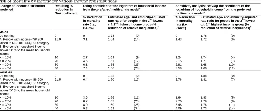
Essay 2 uses multiple cohorts of the National Longitudinal Mortality Study (NLMS) to quantify the absolute income effect on mortality in the United States. Multivariate logistic regressions assess the impact on mortality rate ratios of two hypothetical interventions: lifting everyone living on an equivalized household income at or below the U.S. poverty line in 2000 to the income category just above, and shifting everyone’s income by 10–40% to the mean
larger percentage than overall estimated mortality rates under the same counterfactual redistributions.
Essay 3 uses multiple NLMS cohorts and multilevel Cox proportional hazards regressions to estimate the contextual effect of state-level income inequality on premature mortality in the United States. It uses six different measures of state income inequality, controls for inflation-adjusted, equivalized family income, and adjusts for eight individual-level
To my mother, Mary Helen Stone Brodish, who embodied the virtues of humility, compassion, empathy, caring, and a keen intellect, with which she quietly influenced countless students and acquaintances alike. She treated everyone, no matter their station in life, with the equal respect
that they deserved. She knew nature as a salve for the soul. She lives on in me. “God is the ultimate combined concepts of goodness, kindness, mercy, and love. It is our purpose in life to aspire to that goodness, kindness, mercy and love in our daily deeds and interactions with others. That is what makes us God-fearing. That is what can make us humane.”
ACKNOWLEDGEMENTS
I would like to thank Drs. Mark Holmes and Benjamin Meier for helpful suggestions and advice in drafting Essay 1, and Dr. Bates Buckner for her encouragement. This work was
supported in part by an NIH center grant (R24HD050924) to the Carolina Population Center, the University of North Carolina at Chapel Hill. I would also like to thank Dr. Jahn Hakes at the U.S. Census Bureau for his invaluable assistance in working with the NLMS datasets and in helping me to interpret and apply the resulting outputs for Essays 2 and 3.
PREFACE
Wealth and income inequality have received increasing attention in recent decades. Since the early 1980’s they have steadily increased to extraordinary levels in many societies,
particularly among liberal democratic countries such as the United Kingdom and the United States. These increases have important implications for public health, operationalized herein as HIV prevalence (essay one) and premature mortality (essays two and three), in both developing and developed countries. Among the explanations linking income distribution to population health is the absolute income effect: given that health is a function of income (of course, the reverse is also true), there are diminishing marginal returns of income to health [hi = f (yi), f’ > 0, f” < 0]. The concave shape of the relationship between income and health predicts that, ceteris paribus, more unequal societies have worse average health. Secondly, the contextual effect of income inequality theorizes an additional negative effect on population health from living in a society with high levels of income inequality [hi = f (yi, Gini)]. For example, when incomes of the top 1% pull away from the rest, they cause a variety of “pollution effects” on the quality of life of the bottom 99% (Kawachi & Subramanian, 2014; Subramanian & Kawachi, 2006; Wagstaff & van Doorslaer, 2000).
the work of Hunsmann, Fox, Parkhurst, Shelton, Shandera and others who have been
investigating and tracing the structural drivers of HIV infection and specifically the relationship between wealth distribution and HIV prevalence (Fox, 2010, 2012; Hunsmann, 2009, 2012; Parkhurst, 2010; Shandera, 2007; Shelton, Cassell, & Adetunji, 2005). It was also influenced by my work in the field of program evaluation, in which I have observed how obstacles to
addressing structural drivers extend into our approach to and treatment of global health
problems. For example, proximate causes of disease and health services remedies tend to have favored status over more distal causes and structural remedies, the former being seen as more measureable, actionable, and more in line with our own approaches to population health.
Essay two was suggested as a dissertation topic by Ichiro Kawachi, M.D., Ph.D.,
measure for the United States, as accurately as possible and over a five- to ten-year time period to fully account for lag effects on mortality, the contextual effect of state-level income inequality on premature mortality over and above the absolute income effect. It uses a variety of income inequality indices and a novel approach of proportional hazards multilevel modelling to attempt to discern the presence and magnitude of this effect.
The focus on the distribution (of wealth, income, and mortality) in society and concern for equity takes inspiration from the words of Sir Anthony Atkinson, a preeminent scholar on inequality:
“I was taught, in Cambridge, England, and Cambridge, Massachusetts, to ask, ‘Who gains and who loses?’ from an economic change or policy. This is a question often missing from today’s media discussion and policy debate. Many economic models assume identical representative agents carry out sophisticated decision-making, where distributional issues are suppressed, leaving no space to consider the justice of the resulting outcome. For me, there should be room for such discussion. There is not just one Economics” (Atkinson, 2015) p. 5.
TABLE OF CONTENTS
LIST OF TABLES ... xii
LIST OF FIGURES ... xiv
LIST OF ABBREVIATIONS ... xv
ESSAY 1: AN ASSOCIATION BETWEEN NEIGHBOURHOOD WEALTH INEQUALITY AND HIV PREVALENCE IN SUB-SAHARAN AFRICA ... 1
Introduction ... 1
Conceptual model ... 5
Methods... 6
Data and sample ... 6
Empirical model ... 9
Analysis... 9
Results ... 11
Discussion ... 14
References ... 20
Tables ... 24
ESSAY 2: QUANTIFYING THE INDIVIDUAL-LEVEL ASSOCIATION BETWEEN INCOME AND MORTALITY RISK IN THE UNITED STATES USING THE NATIONAL LONGITUDINAL MORTALITY STUDY ... 29
Introduction ... 29
Methods... 42
Data and Sample ... 42
Empirical model ... 43
Analysis... 44
Results ... 46
Discussion and Conclusion ... 48
References ... 51
Tables ... 56
ESSAY 3: TESTING THE CONTEXTUAL THEORY OF INCOME INEQUALITY IN THE UNITED STATES USING THE NATIONAL LONGITUDINAL MORTALITY STUDY ... 62
Introduction ... 62
Conceptual Model ... 74
Methods... 78
Data and Sample ... 78
Empirical Model ... 79
Analyses ... 81
Results ... 82
Discussion ... 85
References ... 93
Tables ... 98
LIST OF TABLES
Table
1.1. Country sample, sub-Saharan Africa, DHS 2006-2011 ... 24 1.2. Summary statistics for variables included in final model,
by low and high Gini coefficient and wealth ratio ... 25 1.3. Parameter estimates (odds ratios) for three-level models
predicting HIV positive status, Gini coefficient ... 26 1.4. Parameter estimates (odds ratios) for three-level models
predicting HIV positive status, wealth ratio ... 27 1.5. Parameter estimates (odds ratios) for three-level ordered logit
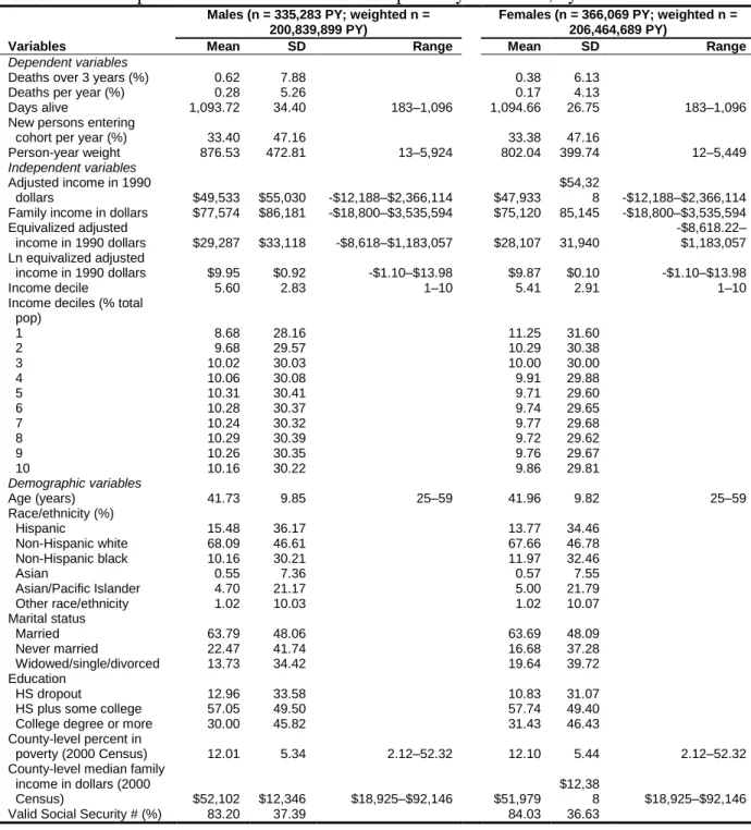
models predicting number of extramarital partners in the past year ... 28 2.1. Descriptive statistics on the 2005-2008 person-year dataset, by sex ... 56 2.2. Person-years, deaths and rate ratios of mortality by equivalized
household income among 25–59-year-old deaths, 2003–2005
cohorts of the NLMS ... 57 2.3. Percentage reductions in overall mortality rates (population
attributable risk percent, PAR%) and changes in the relative
risk of mortality by income for various income redistributions ... 58 3.1. Weighted descriptive statistics for the NLMS (1995 – 2006
cohorts) dataset, by sex ... 98 3.2. Income inequality indices, percent black population and percent
population in poverty, by census region and state, 2000 U.S.
Decennial Census ... 99 3.3. Summary statistics for the state-level variables used in the models,
by sex ... 100 3.4. Hazard ratios for death within 10-year follow-up period, by
income inequality measure and sex ... 101 3.5. Percent change in mortality for a one standard deviation
increase in income inequality, by sex, at the point estimate for
A1. Hazard ratios for death within 10-year follow-up period, by
income inequality measure and sex ... 106 A2. Percent change in mortality for a one standard deviation
increase in income inequality, by sex, at the point estimate for
the beta coefficient, and for the 95% CI for beta ... 107 A3. Hazard ratios for death within 10-year follow-up period,
LIST OF FIGURES
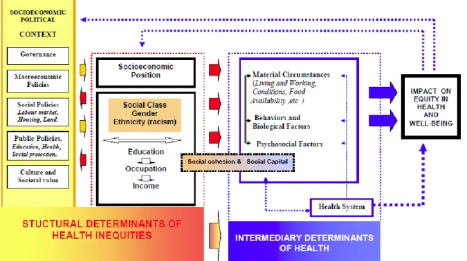
Figure 2.1 - Curvilinear relationship between income and life expectancy ... 59 Figure 2.2 - Final version of the conceptual framework adopted by the WHO
Commission on the Social Determinants of Health ... 60 Figure 2.3 - Density of people per centile of household income, and rate ratios
of mortality (reference group $26,837-$32,446) for various specifications
of the household income variable, 25–59-year-olds, 2003-2005 cohorts ... 61 Figure 3.1 - The contextual effect of income inequality on life expectancy ... 103 Figure 3.2 - Scatterplot of NLMS respondent survival to five years versus
state-level Gini coefficient (males) ... 104 Figure 3.3 - Scatterplots of NLMS respondent survival to five years versus
(a) state-level Palma (90:40) ratio and (b) percentage of state income going to households below the median income (males), with three
LIST OF ABBREVIATIONS
AIC Akaike information criterion
AIDS Acquired immunodeficiency syndrome ASEC Annual Social and Economic Supplement
CI Confidence interval
CPS Current Population Survey
CSDH Commission on the Social Determinants of Health
DC District of Columbia
DHS Demographic and Health Surveys EITC Earned income tax credit
ELISA Enzyme-linked immunosorbent assay
GDP Gross domestic product
GNI Gross national income
HR Hazard ratio
HIV Human immunodeficiency virus
IMF International Monetary Fund
Ln Natural logarithm
MEASURE Monitoring and Evaluation to Assess and Use Results MSA Metropolitan statistical area
NDI National Death Index
NLMS National Longitudinal Mortality Study
OECD Organization for Economic Cooperation and Development
PAR Population attributable risk
PPP Purchasing power parity
PUMS Public Use Microdata Sample
RR Relative risk
SD Standard deviation
SDOH Social determinants of health SEA Statistical enumeration area
SES Socioeconomic status
SSA sub-Saharan Africa
STD Sexually transmitted disease
UNAIDS Joint United Nations Programme on HIV and AIDS
UNU-WIDER United Nations University World Institute for Development Economics Research
ESSAY 1: AN ASSOCIATION BETWEEN NEIGHBOURHOOD WEALTH
INEQUALITY AND HIV PREVALENCE IN SUB-SAHARAN AFRICA1
Introduction
The prevailing explanation for extraordinarily high HIV prevalence rates in parts of sub-Saharan Africa (SSA) employs a behavioral paradigm and emphasizes the high rate of
concurrent sexual partnerships, although there are strongly opposing viewpoints in the literature regarding the role of the latter (Epstein, 2010; Epstein & Morris, 2011; Lurie & Rosenthal, 2010a, 2010b; Mah & Halperin, 2010a; Mah & Halperin, 2010b; Mah & Shelton, 2011; Morris, 2010; Sawers & Stillwaggon, 2010). Donor countries and international aid agencies have
expended enormous effort to try to alter individual sexual behaviors, and only relatively recently has sexual concurrency per se been seriously addressed. Throughout the long history of the regional pandemic both donor and recipient countries have largely neglected the contexts and structural drivers of individual sexual behaviors—some have suggested, for political reasons (Hunsmann, 2009). As Paul Farmer notes in Partner to the Poor, “the failure to contemplate social and economic aspects of epidemics stunts our understanding of them,” making it much more difficult to contain and defeat them (Farmer, 2010; Rosen, 2012).
Although behaviorally-focused prevention appears to have produced recent reductions in HIV incidence rates in the region (Joint United Nations Programme on HIV/AIDS, 2010), it is unclear which interventions have been most effective, nor to what extent. There is clearly a need
1
to better understand the nature and role of network factors such as long-term sexual concurrency, which has been inadequately captured and underreported in sexual behavior surveys, and is at least partially structural in nature because it involves deeply entrenched social and cultural norms (Epstein & Morris, 2011). The heavy toll of the ongoing HIV pandemic in SSA has prompted renewed attention to the social and economic upstream contextual or structural factors,
sometimes termed “the causes of the causes” of disease, which may facilitate viral transmission and undermine intervention effectiveness (Commission on Social Determinants of Health, 2008; Gupta, Parkhurst, Ogden, Aggleton, & Mahal, 2008). In a recent supplement to the Journal of the International AIDS Society devoted entirely to structural drivers of HIV transmission, Seeley
et al. (2012) note elimination of HIV will require “a comprehensive HIV response, that includes meaningful responses to the social, political, economic and environmental factors that affect HIV risk and vulnerability” (Seeley et al., 2012).
Also, a prevailing view emphasizes the role of poverty in the spread of HIV, despite numerous studies demonstrating an inverse relationship between HIV serostatus and poverty status in SSA, which is opposite to the case in the developed world and contrary to common expectations about disease susceptibility and poverty status (Gillespie, Kadiyala, & Greener, 2007; Mishra et al., 2007; Parkhurst, 2010; Shelton et al., 2005). Commenting in the Lancet, Shelton et al. (2005) suggested that both wealth and economic disadvantage may play pivotal roles in HIV transmission through sexual concurrency networks, with wealth being “associated with the mobility, time, and resources to maintain concurrent partnerships” and where women “might improve their economic situation by having more than one concurrent partner” (Shelton et al., 2005) p. 1058. Several investigators have attempted to help resolve the ongoing
explaining the severity of the SSA pandemic. For example, a review by Shandera (2007)
identified several viral, host, transmission, and societal factors that might explain the higher rates of infection in the region (Shandera, 2007). A country-level empirical study by Nattrass (2009) identified a number of social factors associated with HIV prevalence rates, finding little effect of poverty but large and significant effects of the predominant religious affiliation of the country (Nattrass, 2009). Within SSA countries, HIV prevalence rates are generally higher in urban compared to rural areas, but there is also much regional variation, with some poorer, rural areas, such as the Nyanza region of Kenya, having very high prevalence rates. Nattrass et al. (2012) provides an excellent review of the recent literature on the complex interrelationships among poverty, sexual behavior, and HIV in SSA and the methodological challenges inherent in studies attempting to shed light on them. The authors use a panel dataset on young men in Cape Town, South Africa to overcome problems of endogeneity and blunt indicator measurements of sexual behavior, finding important differences by sex (Nattrass, Maughan-Brown, Seekings, &
Whiteside, 2012).
A review by Fox (2010) identified a positive association between HIV prevalence at the country level and the Gini coefficient (a standard measure of economic inequality) among SSA countries (Fox, 2010). These findings suggested a potential association between HIV prevalence and rapid economic development affecting primarily the urban regions of poor developing countries and reflected in rising wealth inequalities, such that it is not poverty or wealth per se, but the level of inequality in a region that predicts HIV prevalence. However, cross-country aggregate-level comparisons are prone to problems such as ecologic fallacy or aggregation bias, and to omitted variable bias from the inability to control for many potentially important
returns to health, then a relationship between health and income is produced at the aggregate level in the absence of a direct effect of economic inequality—the so-called absolute income effect (Gravelle, Wildman, & Sutton, 2002; Kawachi, 2011).
In contrast, the income inequality hypothesis argues that income inequality is an indicator of “social distance” and that greater distance causally leads to greater psychosocial stress and poorer health outcomes (Wilkinson & Pickett, 2009; Wilkinson, 2005; Wilkinson & Pickett, 2006). In the field of economics, this concept implies that “utility” from consumption depends on comparison of one’s own income and consumption to that of others, a concept that has gained recent empirical support in behavioral economics (Fliessbach et al., 2007; Luttmer, 2005). Yet a third “society-wide effects” hypothesis argues that the effects of inequality are related to social capital, trust and social cohesion, with increasing inequality causing reduced cohesion and increased crime and violence (Leigh, Jencks, & Smeeding, 2009). Social heterogeneity, or a social context of varying and potentially competing population preferences and needs, has been linked to the under provision of public goods (Banerjee & Somanathan, 2007).
Using Demographic and Health Surveys (DHS) data from 170 regions across 16
countries, Fox (2012) extended her earlier work by employing multilevel modeling techniques to control for regional-level absolute wealth and a number of individual-level HIV risk factors and establishing an independent association between regional-level wealth inequality and HIV prevalence (Fox, 2012). It has also been noted that the geographic level of the community studied might affect the results of an evaluation of the association between wealth inequality and health outcomes, with support in the literature of a general pattern that the smaller the
comparisons. However, one recent study examined two regions (districts and DHS sampling clusters) simultaneously within one country, Malawi, using a multilevel framework (Durevall & Lindskog, 2012). Specifically, the authors evaluated the effect of district-level consumption inequality and cluster-level (neighborhood) wealth inequality on risk of HIV infection in Malawi women aged 15-24, finding a strong positive association between risk of HIV infection and inequality at both geographic levels, but no association for individual poverty.
The current study builds on these prior efforts by empirically investigating the
relationship between wealth inequality at the statistical enumeration area (SEA) or cluster level within multiple countries in southeastern SSA using the most recent DHS data on HIV
prevalence and several socio-economic and demographic factors. The advantages of this study are that all data within a given country are from the same survey; the number of data points is much larger than previous country-level studies; it examines the inequality-HIV association at a lower level of aggregation (i.e., at the cluster level, compared to the regional or district level) where it has been harder to detect; and two different measures of SEA wealth inequality are utilized as an internal validation of the key independent variable.
Conceptual model
This paper uses ecological systems theory applied to health (or the social ecological model of health). It views individual health status as determined by a broad array of factors operating at multiple levels, often termed macro-, exo-, meso-, and micro-, which describe influences as intercultural, community, organizational, and interpersonal or individual, and has been adopted by World Health Organization’s Commission on the Social Determinants of Health. While this conceptual model applies to general health status, it is utilized here to
threats to population health are infectious disease vulnerability and transmission. HIV is the leading cause of adult mortality in southern SSA and has been responsible for reversing a long-term trend of decreasing mortality rates there. Adult mortality (or, conversely, life expectancy) is a key indicator of population health and directly reflects the general health status of the
population.
As a more direct mechanism of action, researchers theorize that rapid economic
development is associated with rising wealth inequality and reduced social cohesion, leading to the breakdown of traditional family structures. For instance, new opportunities in urban regions may prompt economic migration by male or female household members. They, and those left behind in rural regions, may then take on informal, long-term partners, leading to higher prevalence of HIV in more unequal settings (Fox, 2012). Durevall et al. (2012) note several specific potential links between structural inequality and risk behaviors, particularly transactional sex providing young women and their families the means to remain above subsistence or to improve their economic status (Durevall & Lindskog, 2012). This paper investigates whether HIV prevalence rates are in part determined by such wealth inequities, which reflect differences in social position and levels of social cohesion within a given geographic region (in this case the DHS SEA or cluster), controlling for individual/household wealth and other key individual-level variables.
Methods
Data and sample
higher than 1% as a generalized epidemic (Joint United Nations Program on HIV/AIDS, 2011). Data are downloadable from the MEASURE DHS website at
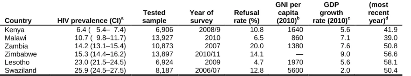
http://www.measuredhs.com/data/available-datasets.cfm. The six countries were: Kenya, Lesotho, Malawi, Swaziland, Zambia, and Zimbabwe. The countries are located in southeastern SSA and have among the highest HIV prevalence rates on the African continent (Table 1.1).
DHS surveys are nationally representative population-based surveys with large sample sizes (usually between 5,000 and 30,000 households). In all households, women age 15-49 are eligible to participate; in many surveys men age 15-54(59) from a sub-sample are also eligible to participate. There are three core questionnaires in DHS surveys: A Household Questionnaire, a Women’s Questionnaire, and a Male questionnaire. HIV biomarker data complements self-reported household survey information by providing an objective profile of a HIV status in the population. The sample is usually based on a stratified two-stage cluster design. The first stage is the SEA (or cluster), generally drawn from Census files. In the second stage, within each SEA, a sample of households is drawn selected from an updated list of households. The sample is generally representative at the national level, residence (urban-rural), and regional (departments, states) levels. This paper evaluates regional or community-level factors (i.e., characteristics of the SEA) that may affect HIV prevalence. Admittedly, the SEA is an arbitrary geographic boundary used only for the purposes of the survey, but it is nevertheless based on Census data and can be aggregated proportionally using the DHS sampling weights so that it should remain representative of the populations under study.
5-10 percent of the negative tests with a second ELISA. For those with discordant results on the two ELISA tests, a new ELISA or a Western Blot is performed (Measure DHS, 2012).
Two key independent variables were created aggregated at the SEA level: 1) the Gini coefficient, representing household wealth inequality, which was constructed using a
transformation of the DHS wealth index score and a Stata user-provided program called FastGini for calculating a weighted Gini-coefficient; 2) a second inequality index using the categories of the DHS categorical wealth index variable: the ratio of the mean wealth of households in the top 20% wealth quintile to that of those in the bottom 20% quintile. I controlled for several key household- or individual-level characteristics, including household wealth quintile (using the DHS-provided household wealth index), frequency of multiple sexual partnerships during the past year and number of lifetime sexual partners, self-reported sexually transmitted infection in the past year, condom use at last intercourse, and several demographic variables associated with HIV serostatus, though it should be recognized that the sexual behavior “controls” were
recognized as potential mediators of the association.
Empirical model
The final empirical model regressed the dependent variable individual HIV serostatus on the two key community-level independent variables (mean cluster-level Gini coefficient and wealth ratio) separately, and included 12 individual-level control variables: number of sexual partners (other than husband/wife) in the past year (dummy-coded as 0, 1, 2, and 3 or more), lifetime number of sexual partners (coded as 1, 2, 3-5, 6-10, and >10), condom use at last intercourse, self-reported STD in the past year, wealth status, male sex, urban residence, age (in years), education level, employed (currently working, having worked in past year, or on leave in the past 7 days), married or living together, and religious affiliation (Catholic, Protestant/other Christian, Muslim, No/other religion).
Multicollinearity was evaluated by examining the correlation matrix for potential control variables included in the final model. I initially evaluated two sexual risk behavior control variables which measured the number of sexual partnerships in the past year. These two variables were the number of sexual partners 1) other than the spouse and 2) including the spouse, during the past year. Because these two variables were correlated above 0.75, I chose a single measure—number of sexual partnerships (other than the spouse) during the past year—as the one providing the best measure of this construct. I also included a measure of number of lifetime sexual partners.
Analysis
needed to account for the hierarchical structure of the data. I used a final multilevel logistic regression model of the form:
logit [Pr (𝐻𝐼𝑉𝑖𝑗𝑘 = 1|𝑋𝑖𝑗𝑘, Ϛ𝑗𝑘, Ϛ𝑘)] = 𝑋𝑖𝑗𝑘′ β + Ϛ𝑗𝑘+ Ϛ𝑘 ,
where Ϛ𝑘|𝑋𝑖𝑗𝑘 ~ 𝑁 (0, ψ) at level 3, and Ϛ𝑗𝑘|𝑋𝑖𝑗𝑘, Ϛ𝑘 ~ 𝑁 (0, ω) at level 2. This model assumed
random variation in the intercepts across clusters and countries (random intercepts model) but constant slopes for the beta coefficients.
The three levels consisted of 43,091 respondents clustered within 2,641 SEAs across six countries. The analysis proceeded in four steps. First, I ran a null or base model including only the dependent variable HIV prevalence to establish the degree of variance at each of the two higher levels in order to validate use of a multilevel framework. Next, I added the level-1 demographic control variables to the model in order to assess the improvement in model fit and presence of significant effects for individual-level predictors of HIV serostatus. Finally, in each of two separate models, I added the key independent variables wealth Gini coefficient and wealth ratio to test for significance of these two predictors, controlling for the individual-level
Results
There were significant differences by low and high values (above and below the median) for both key independent (predictor) variables considered in the model and for most demographic and sexual behavior variables. Table 1.2 indicates these differences, reporting means and standard errors for continuous variables and counts and percentages for categorical variables. Overall, the mean HIV prevalence rate was 17.3%. The mean percent of households in the lowest wealth quintile was 17.2%; the percent of respondents reporting multiple sexual partnerships in the past year was about 29%; the percent reporting condom use at last sex was 22.5%; and the percent reporting an STD in the past year was only 3.8%. Results were remarkably similar for the two measures of wealth inequality (Gini coefficient and wealth ratio), and most comparisons between low and high groups within these two separate inequality measures were statistically significant and largely in the anticipated direction. In these bivariate analyses, higher cluster-level Gini coefficients and wealth ratios were associated with higher HIV prevalence rates and generally with higher rates of risky sexual behaviors.
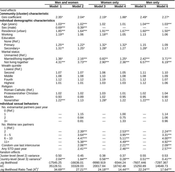
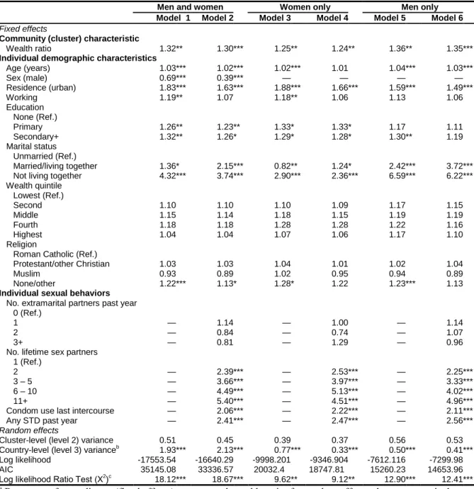
The final multilevel regression models are shown in Table 1.3 (for the Gini coefficient) and Table 1.4 (for the wealth ratio), both for women and men combined and separately for women and men. The coefficients and their patterns in the two tables are remarkably similar. Base models (data not shown) including only the dependent variable HIV prevalence rate showed significant variation by country as anticipated from Table 1.1. In Model 1 of both Table 1.3 and Table 1.4, including the key independent variables cluster-level wealth Gini coefficient and wealth ratio, respectively, and individual-level demographic control variables, both
slightly increased likelihood of being HIV positive. Compared to unmarried persons (the referent group), those who were married or living together were at higher risk and those not living
together were at much higher risk of being HIV positive. Including the cluster-level wealth Gini coefficient and wealth ratio in Model 1 significantly improved the model fit (significant log likelihood ratio test) relative to base models. Both the cluster-level wealth Gini coefficient (OR = 2.35, p < 0.05) and the wealth ratio (OR = 1.32, p < 0.01) were associated with a significant increase in the likelihood of being HIV positive. The marginal effect of the Gini coefficient was that a 1 point increase in the Gini coefficient of an SEA cluster was associated with a 2.35 times increased likelihood of being HIV positive, controlling for all other variables in the model. Similarly, a 1 point increase in the wealth ratio was associated with a 1.3 times increased likelihood of being HIV positive, controlling for the other variables in the model.
Adding in the sexual behavior variables in Model 2 of Tables 1.3 and 1.4 attenuated the effects of both measures of wealth inequality. There was a dose-dependent increase in the odds of being HIV positive with more lifetime sexual partners such that reporting 11 or more partners increased the likelihood of being HIV positive over five-fold. Condom use at last intercourse and an STD in the past year increased this likelihood by two and almost two and-a-half times,
respectively. (Note that because this analysis is correlational, endogeneity or reverse causality probably explains the former association, i.e., condom use is likely to be more frequent among those who know they are HIV positive and/or who engage in higher-risk sex.)
who are married to or living with their partner, controlling for age (which becomes non-significant in Table 1.3). More education among women appears to be slightly protective (decreased odds of HIV infection), whereas it appears to increase risk in the combined men-women models. Also, the odds of HIV infection associated with not living together reduces (from 4.3 to 2.9 times) compared to that for men and women combined. Comparing the full models incorporating the risk behaviors (Model 2 compared to Model 4), again age becomes non-significant and the odds ratio for married/living together again becomes greater than 1, suggesting that risk behaviors are mediating some of this effect and removing any protection associated with cohabitation with sexual partners for women.
Looking at Tables 1.3 and 1.4, Models 5 and 6 for men only, odds ratios for the Gini coefficient and wealth ratio are larger for men. Age is a significant predictor in both reduced and full models, and education appears to increase, rather than decrease risk, although it becomes non-significant in the full models (Model 6 in both tables). It is apparent that the risks associated with cohabitation and not living together (compared to the unmarried referent group) in the combined men-women model is driven by males. The coefficients increase from Model 5 to Model 6 for married/living together for males, suggesting that some other factors increasing risk are not being fully picked up by the risk behaviors.
held for women (OR = 1.54, p < 0.001) but not for men (OR = 1.15); age was not a significant factor in the models for women but was significant and protective in the models for men; urban residence was a significant risk factor for women but not for men; among women, primary education appeared to be a significant risk factor, while a secondary or higher education was no longer significant (compared to models for women and men combined). The risk associated with secondary or higher education appeared to work in opposite directions for men compared to women, reducing risk for women and increasing it for men. Religion was not a significant factor among women but was among men. Among men, being of Protestant or other Christian faith (compared to Catholic) significantly reduced risk, while being of Muslim faith increased it.
Discussion
The relationships between HIV prevalence and the control variables were all in the anticipated direction based on previous studies and expectations about HIV risk and demographic and sexual variables operating at the individual level. Both the cluster-level Gini coefficient for household wealth and the wealth ratio were significant predictors of HIV serostatus, controlling for all other variables in the models, including household wealth and several known behavioral and
demographic predictors of positive serostatus. This is the second known study to produce empirical evidence of these effects using multiple countries and regions in SSA, and the second to demonstrate this effect at the DHS cluster level by utilizing its inherent population-based survey sampling strategy. Although a large literature suggests that economic inequality increases the risk for a variety of diseases after controlling for absolute levels of wealth or income
between regional/district- and/or neighborhood/cluster-level wealth inequality and HIV serostatus after controlling for household-level wealth. Also consistent with these two prior studies, results from models with extramarital partners as the dependent variable suggest that the mechanism is at least in part mediated by an increase in risky sexual behavior.
Consistent with the one prior study of this association at the DHS cluster level in Malawi (Durevall & Lindskog, 2012) but contrary to findings from national-level studies, household wealth was not significantly associated with HIV positive serostatus. This result could be explained by more recent evidence pointing to a complex, dynamic association between wealth and HIV serostatus in SSA. Parkhurst (2010) found that, at the country level, as per capita GDP increased, the confirmed trend for the prevalence of HIV infection to increase with increasing wealth quintile dissipated. He identified a threshold of approximately U.S.$ 2,000 above which this tracking with wealth becomes inconsistent. Half of the countries in the current sample exceeded this GDP threshold. Furthermore, Parkhurst’s analysis of trend data from two Tanzania DHS studies suggested that HIV has become more prevalent in poorer individuals as
The null results for the major religious affiliations could be explained in that most national studies have looked at national-level religious affiliation, and most African Muslim nations are supra-Saharan, where HIV prevalence rates are much lower. Muslims comprised a very small segment of this pooled sample (less than 5%) so the power to detect a significant effect was reduced. However, the direction of the odds ratios suggested a slight protective effect for Muslim religion. The significant effect for “none/other” religious affiliation, which is
attenuated with the addition of the sexual behavior variables to the models, is consistent with the possibility of increased risky-taking behaviors in this minority group in association with lower social status or differential treatment based on religion.
Disaggregation by sex indicated that the relationships between community wealth
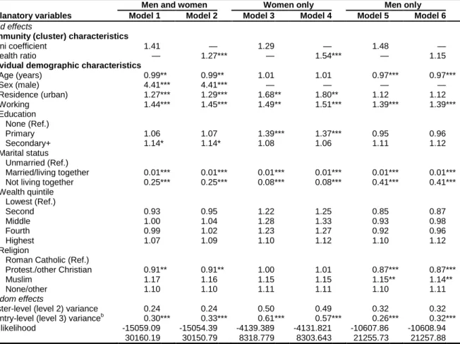
inequality and HIV positive status were stronger for males. However, in the ordered logit models predicting risk behavior (number of extramarital partners in the past year), the wealth ratio was a significant predictor only in models for women. Primary education was a risk, and age was not a risk in models for women (these two reversed in the models for males). Although causality cannot be inferred from these results, taken as a whole, they could be interpreted as suggesting a situation in which neighborhood wealth inequalities, particularly in urbanized areas, are
financial independence. These results point to the importance of disaggregating by sex in such analyses and exploring potential mechanisms of action/causal pathways through modeling behavioral mediators. They are also consistent with the Nattrass et al, 2012 panel study, in which household assets were negatively correlated with HIV status for women but not for men, and in which HIV-positive women were much less likely to have made the transition from (primary) school to tertiary education, a transition which would place them on a trajectory of lowered risk (Nattrass et al., 2012).
It is important to note several study limitations. One methodological limitation is the assumption of constant slopes on the beta coefficients for the two key independent variables. However, adding random slopes to the models would have introduced greater complexity and was not necessary for the purposes of the analysis, and the limited number of countries (six) at level 3 precluded adding this feature at that level. Another likely limitation is violation of basic ordinary least squares logistic regression assumptions through inadequate model specification and the presence of omitted variables, which would bias the beta estimate for the key
independent variables in the direction of a type-1 error. Clearly the final regression model did not capture all variables affecting HIV prevalence at multiple levels and may conflate to some
degree mediation and confounding, but it did capture important available individual-level predictors, and by adding potential behavioral mediators last, I was able to assess the extent to which some variables might mediate the observed effects of the independent variables.
these independent variables has limitations which may lead to erroneous conclusions regarding the direct effect of wealth on HIV status. Because different assets are used in each country to construct the index (although a basic set of assets, such as type of flooring, water supply,
sanitation facilities, appliances, transportation, etc. are included in every survey), it is not directly comparable across countries. Also, the index is not the best proxy for consumption expenditure, the SES measure preferred by economists (Howe, Hargreaves, Gabrysch, & Huttly, 2009). It also tends to negatively weight assets from traditional forms of subsistence production and over-weight assets obtained in the modern cash economy, and thus tends to capture involvement in the modern, cash-oriented economy, which is also highly correlated with both urbanization and education level (Bingenheimer, 2007). This property may help explain its consistent positive association with HIV status among poorer developing African countries. However, the DHS index is considered a reasonable measure of economic well-being, it is the measure that was available in the datasets, and its major purpose was to construct within-cluster relative measures of economic inequality and to control for absolute measures of individual wealth status rather than to compare wealth status across countries.
Also, because these data are cross-sectional, we can only observe the relationship between wealth inequality and HIV prevalence at a single point in time. Reverse causality, in which HIV infection affects household wealth and cluster-level wealth distribution, is
results point to some of the difficulties in doing empirical work in the field of social/structural determinants of health. It is often difficult to relate macro-level social factors to individual health status due to unavailability of accurate measures of both micro- and macro-level factors, and to the complexity of methodologies needed to adequately control for factors operating at multiple levels. Nevertheless, neglect of these higher-level factors moderating individual behaviors risks ascribing too much predictive power to micro-level factors and may lead to missed opportunities to modify social environments and create structural changes which induce more
REFERENCES
Atkinson, A. B. (2015). Introduction Inequality: What can be done? Cambridge, MA: Harvard University Press.
Banerjee, A., & Somanathan, R. (2007). The political economy of public goods: Some evidence from India. Journal of Development Economics, 82(2), 287-314.
Bingenheimer, J. B. (2007). Wealth, Wealth Indices and HIV Risk in East Africa. International Family Planning Perspectives, 33(2), 83-84.
Commission on Social Determinants of Health. (2008). Closing the gap in a generation: health equity through action on the social determinants of health. Final Report of the
Commission on Social Determinants of Health. Retrieved from Geneva, Switzerland:
http://www.who.int/social_determinants/thecommission/finalreport/en/index.html
Durevall, D., & Lindskog, A. (2012). Economic Inequality and HIV in Malawi. World Development, 40(7), 1435-1451.
Epstein, H. (2010). The mathematics of concurrent partnerships and HIV: a commentary on Lurie and Rosenthal. AIDS and Behavior, 14, 29-30.
Epstein, H., & Morris, M. (2011). Concurrent partnerships and HIV: an inconvenient truth. Journal of the International AIDS Society, 14(1), 13. Retrieved from
http://www.jiasociety.org/content/14/1/13
Farmer, P. (2010). Partner to the Poor: A Paul Farmer Reader. Berkeley and Los Angeles: University of California Press.
Fliessbach, K., Weber, B., Trautner, P., Dohmen, T., Sunde, U., Elger, C. E., & Falk, A. (2007). Social comparison affects reward-related brain activity in the human ventral striatum. Science, 318(5854), 1305-1308.
Fox, A. M. (2010). The Social Determinants of HIV Serostatus in Sub-Saharan Africa: An Inverse Relationship Between Poverty and HIV? Public Health Reports, 125, 16-24. Fox, A. M. (2012). The HIV–poverty thesis re-examined: Poverty, wealth, or inequality as a
social determinant of HIV infection in sub-Saharan Africa? Journal of Biosocial Science, 44(04), 459-480.
Gillespie, S., Kadiyala, S., & Greener, R. (2007). Is poverty or wealth driving HIV transmission? AIDS, 21, S5-S16.
Gupta, G. R., Parkhurst, J. O., Ogden, J. A., Aggleton, P., & Mahal, A. (2008). HIV prevention 4 - Structural approaches to HIV prevention. Lancet, 372(9640), 764-775.
Howe, L. D., Hargreaves, J. R., Gabrysch, S., & Huttly, S. R. A. (2009). Is the wealth index a proxy for consumption expenditure? A systematic review. Journal of Epidemiology and Community Health, 63(11), 871-877.
Hunsmann, M. (2009). Political determinants of variable aetiology resonance: explaining the African AIDS epidemics. International Journal of STD & AIDS, 20(12), 834-838. Hunsmann, M. (2012). Limits to evidence-based health policymaking: Policy hurdles to
structural HIV prevention in Tanzania. Social Science & Medicine, 74(10), 1477-1485. Joint United Nations Program on HIV/AIDS. (2011). UNAIDS Terminology Guidelines.
Retrieved from
http://www.unaids.org/en/media/unaids/contentassets/documents/unaidspublication/2011/ JC2118_terminology-guidelines_en.pdf
Joint United Nations Programme on HIV/AIDS. (2010). MDG6: Six things you need to know about the AIDS response today. Retrieved from Geneva:
http://data.unaids.org/pub/Report/2010/20100917_mdg6_report_en.pdf
Kawachi, I. (2011, April 5, 2011). Income inequality and population health. Sulzberger Distinguished Lecture Series. Retrieved from
http://www.childandfamilypolicy.duke.edu/events_detail.php?id=56
Kawachi, I. (2014). [Personal Communication].
Kawachi, I., & Subramanian, S. V. (2014). Income Inequality. In I. K. Lisa F. Berkman, M. Maria Glymour (Ed.), Social Epidemiology (Second ed., pp. 126-152). New York: Oxford University Press.
Leigh, A., Jencks, C., & Smeeding, T. M. (2009). Health and Economic Inequality. In W.
Salverda, B. Nolan, & T. Smeeding (Eds.), The Oxford Handbook of Economic Inequality (pp. 384-405). Oxford, UK: Oxford University Press.
Lurie, M., & Rosenthal, S. (2010a). The Concurrency Hypothesis in Sub-Saharan Africa:
Convincing Empirical Evidence is Still Lacking. Response to Mah and Halperin, Epstein, and Morris. AIDS and Behavior, 14, 34-37.
Lurie, M., & Rosenthal, S. (2010b). Concurrent Partnerships as a Driver of the HIV Epidemic in Sub-Saharan Africa? The Evidence is Limited. AIDS and Behavior, 14, 17 - 24.
Mah, T., & Halperin, D. (2010). Concurrent Sexual Partnerships and the HIV Epidemics in Africa: Evidence to Move Forward. AIDS and Behavior, 14(1), 11-16.
doi:10.1007/s10461-008-9433-x
Mah, T., & Halperin, D. (2010). The Evidence for the Role of Concurrent Partnerships in Africa's HIV Epidemics: A Response to Lurie and Rosenthal. AIDS and Behavior, 14, 25-28.
Mah, T., & Shelton, J. (2011). Concurrency revisited: increasing and compelling epidemiological evidence. Journal of the International AIDS Society, 14(1), 33. Retrieved from
http://www.jiasociety.org/content/14/1/33
Measure DHS. (2012). DHS Overview: HIV Prevalence. Retrieved from
http://www.measuredhs.com/topics/HIV-Corner/hiv-prev/index.cfm
Mishra, V., Assche, S. R. V., Greener, R., Vaessen, M., Hong, R., Ghys, P. D., . . . Rutstein, S. (2007). HIV infection does not disproportionately affect the poorer in sub-Saharan Africa. AIDS, 21, S17-S28.
Morris, M. (2010). Barking up the Wrong Evidence Tree. Comment on Lurie & Rosenthal, "Concurrent Partnerships as a Driver of the HIV Epidemic in Sub-Saharan Africa? The Evidence is Limited". AIDS and Behavior, 14, 31-33.
Nattrass, N. (2009). Poverty, Sex and HIV. AIDS and Behavior, 13(5), 833-840.
Nattrass, N., Maughan-Brown, B., Seekings, J., & Whiteside, A. (2012). Poverty, sexual
behaviour, gender and HIV infection among young black men and women in Cape Town, South Africa. African Journal of AIDS Research, 11(4), 307-317.
Parkhurst, J. O. (2010). Understanding the correlations between wealth, poverty and human immunodeficiency virus infection in African countries. Bulletin of the World Health Organization, 88(7), 519-526.
Phelan, J. C., Link, B. G., & Tehranifar, P. (2010). Social Conditions as Fundamental Causes of Health Inequalities: Theory, Evidence, and Policy Implications. Journal of Health and Social Behavior, 51, S28-S40.
Rosen, D. (2012, April 27, 2012 ). Social Networks of Disease: ‘Tinderbox,’ by Craig Timberg and Daniel Halperin. New York Times Sunday Book Review.
Sahn, D. E., & Stifel, D. C. (2003). Urban-rural inequality in living standards in africa. Journal of African Economies, 12(4), 564-597.
Seeley, J., Watts, C. H., Kippax, S., Russell, S., Heise, L., & Whiteside, A. (2012). Addressing the structural drivers of HIV: a luxury or necessity for programmes? Journal of the International AIDS Society, 15(Suppl 1), 17397.
doi:http://dx.doi.org/10.7448/IAS.15.3.17397
Shandera, W. X. (2007). Key determinants of AIDS impact in Southern sub-Saharan Africa. AJAR-African Journal of Aids Research, 6(3), 271-286.
Shelton, J. D., Cassell, M. M., & Adetunji, J. (2005). Is poverty or wealth at the root of HIV? The Lancet, 366(9491), 1057-1058. doi: http://dx.doi.org/10.1016/S0140-6736(05)67401-6
Subramanian, S. V., & Kawachi, I. (2004). Income inequality and health: What have we learned so far? Epidemiologic Reviews, 26, 78-91.
Subramanian, S. V., & Kawachi, I. (2006). Being well and doing well: on the importance of income for health. International Journal of Social Welfare, 15, S13-S22.
Wagstaff, A., & van Doorslaer, E. (2000). Income inequality and health: What does the literature tell us? Annual Review of Public Health, 21, 543-567.
Wai-Poi, M., Spilerman, S., & Torche, F. (2008). Economic well-being: Concepts and measurement using Asset Indices.
Wilkinson, R., & Pickett, K. E. (2009). The Spirit Level: Why More Equal Societies Almost Always Do Better: Penguin.
Wilkinson, R. G. (2005). The Impact of Inequality: How to Make Sick Societies Healthier. New York: New Press.
TABLES
Table 1.1. Country sample, sub-Saharan Africa, DHS 2006-2011
Country HIV prevalence (CI)a
Tested sample
Year of survey
Refusal rate (%)
GNI per capita (2010)b
GDP growth rate (2010)c
Gini ratio (most recent year)d
Kenya 6.4 ( 5.4– 7.4) 6,906 2008/9 10.8 1640 5.6 41.9
Malawi 10.7 ( 9.8–11.7) 13,927 2010 6.5 860 7.1 39.0
Zambia 14.2 (13.1–15.4) 10,873 2007 20.0 1380 7.6 50.8
Zimbabwe 15.3 (14.4–16.2) 13,897 2010/11 14.1 — 9.0 56.6
Lesotho 23.0 (21.5–24.5) 6,924 2009 4.7 1970 5.6 58.1
Swaziland 25.9 (24.5–27.5) 8,187 2006/07 12.8 5600 2.0 50.4
a Countries ordered from lowest to highest prevalence. Figures weighted for probability of selection into the sample. b
GNI per capita, PPP (purchasing power parity, current international $), 2010. Zimbabwe’s data missing due to the ongoing political and economic crisis; data from World Bank, World Development Indicators Database.
c Annual GDP growth rate for 2010. Data from World Bank, World Development Indicators Database. d
Table 1.2. Summary statistics for variables included in final model, by low and high Gini coefficient and wealth ratio
Gini coefficient Wealth ratio
Total Low High Low High
n 43,032a 21,520 21,512 21,522 21,509
Dependent variable
HIV positive, n (%) 7,444 (17.3) 3,395 (15.8) 4,048 (18.8) *** 3,347 (15.6) 4,097 (19.0) ***
Independent variables
Gini coefficient, mean (SE) 0.42 (0.004) 0.28 (0.003) 0.56 (0.003) *** 0.34 (0.006) 0.50 (0.004) ***
Wealth ratio, mean (SE) 1.49 (0.008) 1.35 (0.009) 1.62 (0.012) *** 1.23 (0.003) 1.74 (0.011) ***
Demographic variables
Age in years, mean (SE) 30.8 (0.06) 31.1 (0.09) 30.5 (0.08) *** 31.1 (0.09) 30.5 (0.08) ***
Male, n (%) 20,403 (47.4) 10,337 (48.0) 10,066 (46.8) * 10,421 (48.4) 9,982 (46.4) ***
Urban residence 12,273 (28.5) 7,808 (36.3) 4,465 (20.8) *** 8,540 (40.0) 3,733 (17.4) ***
Working 30,916 (71.8) 15,893 (73.8) 15,023 (69.8) *** 15,954 (74.1) 14,962 (69.6) ***
Education
None 3,348 ( 7.8) 1,993 ( 9.3) 1,355 ( 6.3) *** 1,591 ( 7.4) 1,757 ( 8.2)
Primary 20,418 (47.4) 10,105 (47.0) 10,313 (47.9) 9,611 (44.6) 10,807 (50.2) ***
Secondary+ 16,650 (38.7) 7,699 (35.8) 8,951 (41.6) *** 8,651 (40.2) 7,998 (37.2) **
Wealth quintile
Lowest 7,380 (17.2) 4,819 (22.4) 2,561 (11.9) *** 3,504 (16.3) 3,876 (18.0)
Second 7,940 (18.4) 3,953 (18.4) 3,988 (18.5) 3,739 (17.4) 4,201 (19.5) *
Middle 8,386 (19.5) 2,892 (13.4) 5,494 (25.5) *** 3,826 (17.8) 4,560 (21.2) ***
Fourth 9,284 (21.6) 3,429 (15.9) 5,855 (27.2) *** 4,352 (20.2) 4,932 (22.9) *
Highest 10,041 (23.3) 6,428 (29.9) 3,613 (16.8) *** 6,101 (28.4) 3,940 (18.3) ***
Marital status
Unmarried 8,363 (19.4) 3,935 (18.3) 4,428 (20.6) ** 3,624 (16.8) 4,739 (22.0) ***
Married/living together 31,888 (74.1) 16,260 (75.6) 15,628 (72.6) *** 16,504 (76.7) 15,384 (71.5) ***
Not living together 2,780 ( 6.5) 1,325 ( 6.2) 1,455 ( 6.8) * 1,394 ( 6.5) 1,386 ( 6.4)
Religion
Roman Catholic 8,369 (19.4) 4,452 (20.7) 3,917 (18.2) ** 4,149 (19.3) 4,220 (19.6)
Protestant/other Christian 27,131 (63.0) 13,961 (64.9) 13,170 (61.2) *** 14,578 (67.7) 12,553 (58.4) ***
Muslim 1,793 ( 4.2) 947 ( 4.4) 846 ( 3.9) 818 ( 3.8) 975 ( 4.5)
None/other 5,739 (13.3) 2,160 (10.0) 3,579 (16.6) *** 1,978 (9.2) 3,762 (17.5) ***
Sexual behavior variables
No. extramarital sex partners past year
0 30,684 (71.3) 15,661 (72.8) 15,023 (69.8) ** 15,979 (74.2) 14,705 (68.4) ***
1 10,463 (24.3) 5,007 (23.3) 5,456 (25.4) ** 4,722 (21.9) 5,741 (26.7) ***
2 1,531 ( 3.6) 669 ( 3.1) 862 ( 4.0) *** 645 ( 3.0) 886 (4.1) ***
3+ 354 ( 0.8) 183 ( 0.9) 171 ( 0.8) 177 ( 0.8) 177 (0.8)
No. lifetime sex partners
1 13,653 (31.7) 6,809 (31.6) 6,844 (31.8) 6,918 (32.1) 6,735 (31.3)
2 9,946 (23.1) 4,960 (23.0) 4,986 (23.2) 4,888 (22.7) 5,058 (23.5)
3 - 5 12,339 (28.7) 6,083 (28.3) 6,256 (29.1) 6,018 (28.0) 6,321 (29.4) *
6 - 10 3,864 ( 9.0) 2,027 ( 9.4) 1,837 ( 8.5) * 2,028 ( 9.4) 1,836 ( 8.5) *
11+ 3,229 ( 7.5) 1,641 ( 7.6) 1,588 ( 7.4) 1,670 ( 7.8) 1,559 ( 7.2)
Condom use last sex 9,697 (22.5) 4,477 (20.8) 5,220 (24.3) *** 4,315 (20.0) 5,382 (25.0) ***
STD past year 1,624 ( 3.8) 738 ( 3.4) 887 ( 4.1) ** 717 ( 3.3) 907 ( 4.2) ***
a Estimated population size adjusted for survey sampling frame.
Table 1.3. Parameter estimatesa (odds ratios) for three-level models predicting HIV positive status, Gini coefficient
Men and women Women only Men only
Model 1 Model 2 Model 3 Model 4 Model 5 Model 6
Fixed effects
Community (cluster) characteristic
Gini coefficient 2.35 * 2.04 * 2.19 * 1.88 * 2.49 * 2.27 *
Individual demographic characteristics
Age (years) 1.03 *** 1.02 *** 1.02 1.01 1.04 *** 1.03 ***
Sex (male) 0.69 *** 0.39 *** — — — —
Residence (urban) 1.85 *** 1.64 *** 1.91 *** 1.67 *** 1.60 *** 1.50 **
Working 1.19 ** 1.06 1.18 ** 1.05 1.13 1.06
Education
None (Ref.)
Primary 1.25 ** 1.22 * 1.32 * 1.32 * 1.15 1.09
Secondary+ 1.31 ** 1.25 * 1.28 * 1.27 1.28 * 1.17
Marital status
Unmarried (Ref.)
Married/living together 1.36 * 2.16 *** 0.82 ** 1.25 * 2.42 *** 3.71 ***
Not living together 4.31 *** 3.73 *** 2.90 *** 2.36 *** 6.57 *** 6.19 ***
Wealth quintile
Lowest (Ref.)
Second 1.07 1.07 1.06 1.05 1.11 1.10
Middle 1.08 1.08 1.10 1.08 1.08 1.09
Fourth 1.12 1.12 1.19 1.21 1.12 1.07
Highest 1.01 1.01 1.03 1.03 1.12 1.06
Religion
Roman Catholic (Ref.)
Protestant/other Christian 1.02 1.02 1.03 1.01 1.02 1.04
Muslim 0.93 0.89 1.02 0.95 0.95 0.90
None/other 1.22 *** 1.13 1.28 * 1.22 1.22 *** 1.12
Individual sexual behaviors
No. extramarital partners past year
0 (Ref.)
1 — 1.15 — 1.00 — 1.14
2 — 0.84 — 0.75 — 1.06
3+ — 0.81 — 1.33 — 0.96
No. lifetime sex partners
1 (Ref.)
2 — 2.39 *** — 2.53 *** — 2.24 ***
3 – 5 — 3.64 *** — 3.95 *** — 3.31 ***
6 – 10 — 4.47 *** — 5.11 *** — 4.00 ***
11+ — 5.38 *** — 4.49 *** — 4.92 ***
Condom use last intercourse — 2.06 *** — 2.21 *** — 2.09 ***
Any STD past year — 2.41 *** — 2.46 *** — 2.57 ***
Random effects
Cluster-level (level 2) variance 0.50 0.45 0.38 0.37 0.55 0.53
Country-level (level 3) varianceb 2.04 *** 1.84 *** 0.56 *** 0.28 *** 0.51 *** 0.41 ***
Log likelihood -17545.25 -16636.01 -9990.919 -9344.24 -7607.446 -7297.367
AIC 35128.51 33328.03 20017.84 18742.48 15250.89 14648.73
Log likelihood Ratio Test (Χ2)c 34.69 *** 27.21 *** 24.18 *** 14.44 *** 22.24 *** 17.64 ***
a Parameters for predictors (fixed effects) are reported as odds ratio; for random effects, the parameter is the
variance.
b Significance of random effects evaluated by comparing model with a similar one in which random effects have
been constrained to be zero.
c Compared with model excluding the independent variable.
Table 1.4. Parameter estimatesa (odds ratios) for three-level models predicting HIV positive status, wealth ratio
Men and women Women only Men only
Model 1 Model 2 Model 3 Model 4 Model 5 Model 6
Fixed effects
Community (cluster) characteristic
Wealth ratio 1.32 ** 1.30 *** 1.25 ** 1.24 ** 1.36 ** 1.35 ***
Individual demographic characteristics
Age (years) 1.03 *** 1.02 *** 1.02 *** 1.01 1.04 *** 1.03 ***
Sex (male) 0.69 *** 0.39 *** — — — —
Residence (urban) 1.83 *** 1.63 *** 1.88 *** 1.66 *** 1.59 *** 1.49 ***
Working 1.19 ** 1.07 1.18 ** 1.06 1.13 1.06
Education
None (Ref.)
Primary 1.26 ** 1.23 ** 1.33 * 1.33 * 1.17 1.11
Secondary+ 1.32 ** 1.26 * 1.29 * 1.28 * 1.30 ** 1.19
Marital status
Unmarried (Ref.)
Married/living together 1.36 * 2.15 *** 0.82 ** 1.24 * 2.42 *** 3.72 ***
Not living together 4.32 *** 3.74 *** 2.90 *** 2.36 *** 6.59 *** 6.22 ***
Wealth quintile
Lowest (Ref.)
Second 1.10 1.10 1.10 1.09 1.17 1.15
Middle 1.15 1.14 1.18 1.15 1.19 1.19
Fourth 1.18 1.18 1.28 1.28 1.22 1.16
Highest 1.04 1.04 1.07 1.06 1.17 1.10
Religion
Roman Catholic (Ref.)
Protestant/other Christian 1.03 1.03 1.04 1.01 1.02 1.04
Muslim 0.93 0.89 1.02 0.95 0.94 0.89
None/other 1.22 *** 1.13 * 1.28 * 1.22 1.23 *** 1.13
Individual sexual behaviors
No. extramarital partners past year
0 (Ref.)
1 — 1.14 — 1.00 — 1.14
2 — 0.84 — 0.74 — 1.07
3+ — 0.81 — 1.29 — 0.96
No. lifetime sex partners
1 (Ref.)
2 — 2.39 *** — 2.53 *** — 2.25 ***
3 – 5 — 3.66 *** — 3.97 *** — 3.33 ***
6 – 10 — 4.49 *** — 5.13 *** — 4.02 ***
11+ — 5.40 *** — 4.51 *** — 4.96 ***
Condom use last intercourse — 2.06 *** — 2.22 *** — 2.11 ***
Any STD past year — 2.41 *** — 2.47 *** — 2.56 ***
Random effects
Cluster-level (level 2) variance 0.51 0.45 0.39 0.37 0.56 0.53
Country-level (level 3) varianceb 1.93 *** 2.13 *** 0.77 *** 0.33 *** 0.50 *** 0.41 ***
Log likelihood -17553.54 -16640.29 -9998.201 -9346.904 -7612.116 -7299.98
AIC 35145.08 33336.57 20032.4 18747.81 15260.23 14653.96
Log likelihood Ratio Test (Χ2)c 18.12 *** 18.67 *** 9.62 ** 9.12 ** 12.90 *** 12.41 ***
a Parameters for predictors (fixed effects) are reported as odds ratio; for random effects, the parameter is the
variance.
b Significance of random effects evaluated by comparing model with a similar one in which random effects have
been constrained to be zero.
c Compared with model excluding the independent variable.
Table 1.5. Parameter estimatesa (odds ratios) for three-level ordered logit models predicting number of extramarital partners in the past year
Men and women Women only Men only
Explanatory variables Model 1 Model 2 Model 3 Model 4 Model 5 Model 6
Fixed effects
Community (cluster) characteristics
Gini coefficient 1.41 — 1.29 — 1.48 —
Wealth ratio — 1.27 *** — 1.54 *** — 1.15
Individual demographic characteristics
Age (years) 0.99 ** 0.99 ** 1.01 1.01 0.97 *** 0.97 ***
Sex (male) 4.41 *** 4.41 *** — — — —
Residence (urban) 1.27 *** 1.29 *** 1.68 ** 1.80 ** 1.12 1.12
Working 1.44 *** 1.45 *** 1.49 ** 1.51 *** 1.39 *** 1.39 ***
Education
None (Ref.)
Primary 1.06 1.07 1.39 *** 1.37 *** 0.95 0.96
Secondary+ 1.14 * 1.14 * 1.08 1.06 1.11 1.12
Marital status
Unmarried (Ref.)
Married/living together 0.01 *** 0.01 *** 0.01 *** 0.01 *** 0.01 *** 0.01 ***
Not living together 0.25 *** 0.25 *** 0.08 *** 0.08 *** 0.41 *** 0.41 ***
Wealth quintile
Lowest (Ref.)
Second 0.93 0.95 1.22 1.25 0.85 0.87
Middle 1.00 1.04 1.28 1.33 0.93 0.98
Fourth 0.99 1.02 1.23 1.27 0.92 0.96
Highest 1.07 1.09 1.10 1.12 1.10 1.12
Religion
Roman Catholic (Ref.)
Protest./other Christian 0.91 ** 0.91 ** 1.00 1.01 0.87 *** 0.87 ***
Muslim 1.17 1.16 1.15 1.15 1.15 ** 1.14 **
None/other 1.10 1.10 1.11 1.11 1.10 1.11
Random effects
Cluster-level (level 2) variance 0.24 0.24 0.50 0.49 0.32 0.32
Country-level (level 3) varianceb 0.30 *** 0.33 *** 0.61 *** 0.57 *** 0.26 *** 0.32 ***
Log likelihood -15059.09 -15054.39 -4139.389 -4131.821 -10607.86 -10608.94
AIC 30160.19 30150.79 8318.779 8303.643 21255.73 21257.88
a Parameters for predictors (fixed effects) are reported as odds ratio; for random effects, the parameter is the
variance.
b
Significance of random effects evaluated by comparing model with a similar one in which random effects have been constrained to be zero.
ESSAY 2: QUANTIFYING THE INDIVIDUAL-LEVEL ASSOCIATION BETWEEN INCOME AND MORTALITY RISK IN THE UNITED STATES USING THE
NATIONAL LONGITUDINAL MORTALITY STUDY
Occurrent, quod genus egestatis gravissimum est, in divitiis inopes.2
Introduction
Evidence to date, albeit from a relatively limited number of experimental or quasi-experimental studies, supports the conclusion that income poverty has an adverse causal impact on health. In a recent review of the evidence from social epidemiology, Glymour and colleagues discuss the difficulties of establishing a causal relationship due to reverse causation and to factors jointly determining income and health (Glymour, Avendano, & Kawachi, 2014). There is a tendency for social epidemiologists to view the relationship as causal from income to health: more income means greater ability to purchase good housing, food, clothing, and other health-generating goods. But those employing a health capital theoretical orientation stemming from human capital theory or the Grossman model (Grossman, 1972) tend to see the causal
relationship going from health to income, or at least as more bi-directional. Particularly useful in understanding relationships between employment and health, the Grossman model views
individuals as both consumers and producers of health: health is both a consumption good providing direct utility, and an investment good increasing productivity, reducing time in
2“To be poor in a wealthy society is the worst kind of poverty.” Lucius Annaeus Seneca.
sickness, and increasing income. The individual derives utility from his/her health stock, consumption of other goods, and leisure time.
Experimental and quasi-experimental studies addressing the income health relationship have fallen into two main categories. First, randomized experiments assign one group of individuals or households to some form of income transfer, compared to a control group not assigned a transfer. Second, natural experiments assign income exogenously or “as-if-random” due to such “shocks” as a change in entitlement laws, lottery winnings, or stock market
windfalls. Overall, the results of this literature suggest that policy-induced change via conditional cash transfers that require human capital investments have significant positive health effects on mothers and children, and that income shocks in the first five years of life, compared to other points in the life course, have the largest effects on health (Glymour et al., 2014). Long-term or permanent increases in income appear to yield positive health benefits, based on evaluations of intermediate outcomes such as child developmental milestones and school enrollment, but there is a need for evidence on long-term, sustained health improvements. Additionally, total costs of programmatic interventions must be considered, because in the final analysis, if income
improves health, then the cost of potential health interventions of any description must be weighed against the alternative of simply giving program beneficiaries the money directly, as with social cash transfers (Glymour et al., 2014).
Shonkoff & Levitt, 2010) and are targetable through early interventions (Mercy & Saul, 2009). In particular, Shonkoff and colleagues have developed a biodevelopmental framework for understanding the origins of disparities in learning, behavior, and health based on evolutionary biology and recent scientific advances in understanding of gene-environment interactions. He cites a 2007 Lancet series on child development in low-income countries, which estimates that 200 million children worldwide are not reaching their cognitive potential due to deep poverty and its associated toxic stress (Grantham-McGregor et al., 2007; Shonkoff, 2010). In the United States, with a childhood poverty rate of nearly 20 percent, there is ample scope for moving public policy forward to close “the gap between what we know and what we do to promote the healthy development of young children” (Shonkoff, 2010).
The above framework is necessarily highly interdisciplinary. Raphael reviews the large number of disciplinary perspectives involved in understanding the association between poverty in childhood and adverse health outcomes in adulthood, and in doing something about it (Raphael, 2011). These disciplinary perspectives include political science, political economy, sociology, and institutions (e.g., the coevolution and collective action literature), but also societal discourses/explanations/rationalizations to justify tolerating such high levels of childhood
should be recognized and promoted. It should also be mentioned that the development economist Amartya Sen was instrumental in setting up the World Health Organization Commission on Social Determinants of Health (WHO CSDH) and was one of its members. There is a close affinity between his ethical arguments for viewing social justice as the expansion of freedoms and social epidemiological research on the effects on health of having control, autonomy, and full participation in social relationships (Sen, 2000, 2008; Venkatapuram, Bell, & Marmot, 2010).