COUPLED DICTIONARY LEARNING FOR IMAGE ANALYSIS
Tian Cao
A dissertation submitted to the faculty of the University of North Carolina at Chapel Hill in partial fulfillment of the requirements for the degree of Doctor of Philosophy in the Department of
Computer Science.
Chapel Hill 2016
©2016 Tian Cao
ABSTRACT
Tian Cao: COUPLED DICTIONARY LEARNING FOR IMAGE ANALYSIS (Under the direction of Marc Niethammer)
Modern imaging technologies provide different ways to visualize various objects ranging from molecules in a cell to the tissue of a human body. Images from different imaging modalities reveal distinct information about these objects. Thus a common problem in image analysis is how to relate different information about the objects. For instance, relating protein locations from fluorescence microscopy and the protein structures from electron microscopy. These problems are challenging due to the difficulties in modeling the relationship between the information from different modalities.
ACKNOWLEDGEMENTS
I would like to express my sincere gratitude to my advisor, Marc Niethammer, for introducing me to the world of medical image analysis and for keeping me motivated with his great enthusiasm for the subject. I have continuously benefited from his knowledge, his encouragement and his personal guidance.
I would also like to thank my committee members, Alexander C. Berg, Klaus M. Hahn, Martin Styner and Vladimir Jojic, for their feedback and advice.
Additionally, I would like to thank my labmates for their help and support: Liang Shan, Yang Huang, Istvan Csapo, Yi Hong, Xiao Yang, Heather Couture, Xu Han, Nikhil Singh, Thomas Polzin.
TABLE OF CONTENTS
LIST OF TABLES . . . x
LIST OF FIGURES . . . xiii
LIST OF ABBREVIATIONS . . . xix
1 INTRODUCTION . . . 1
1.1 Motivations . . . 1
1.1.1 Multi-modal image registration for correlative microscopy . . . 1
1.1.2 Deformation estimation from appearances . . . 2
1.1.3 Coordination between GTPase activities and cell movements . . . 3
1.1.4 Coupled dictionary learning . . . 4
1.1.5 Robust coupled dictionary learning . . . 4
1.2 Contributions . . . 5
1.3 Thesis statement. . . 5
1.4 Outline . . . 6
2 BACKGROUND . . . 7
2.1 Image registration . . . 7
2.2 Image analogy . . . 9
2.2.1 Nearest neighbor search . . . 10
2.3 Sparse representation . . . 12
2.4 Dictionary learning . . . 13
2.4.1 Data preprocessing . . . 14
2.5 Coupled dictionary learning . . . 15
2.5.1 Standard coupled dictionary learning (CDL) . . . 16
2.5.2 Semi-coupled dictionary learning (SCDL) . . . 16
2.5.3 Numerical solution . . . 17
2.6 Conclusion . . . 18
3 COUPLED DICTIONARY LEARNING FOR MULTI-MODAL REGISTRATION . . . 19
3.1 Introduction . . . 19
3.2 Related work . . . 22
3.2.1 Multi-modal image registration for correlative microscopy . . . 22
3.2.2 Image synthesis . . . 23
3.3 Method . . . 24
3.3.1 CDL for image analogies . . . 24
3.3.2 Numerical solution . . . 25
3.3.3 Intensity normalization . . . 26
3.3.4 Use in multi-modal image registration . . . 27
3.4 Results. . . 27
3.4.1 Data . . . 27
3.4.2 Registration of SEM/confocal images (with fiducials) . . . 28
3.4.2.1 Data preparation . . . 28
3.4.2.2 Image analogy (IA) results . . . 28
3.4.2.3 Image registration results . . . 32
3.4.2.4 Hypothesis test on registration results . . . 34
3.4.2.5 Discussion . . . 37
3.4.3 Registration of TEM/confocal images (without fiducials) . . . 37
3.4.3.1 Data preparation . . . 37
3.4.3.3 Image registration results . . . 38
3.4.3.4 Hypothesis test on registration results . . . 41
3.4.3.5 Discussion . . . 44
3.5 Conclusion . . . 44
4 SEMI-COUPLED DICTIONARY LEARNING FOR DEFORMATION ESTIMATION . . 46
4.1 Introduction . . . 46
4.2 Method . . . 48
4.2.1 SCDL for deformations and appearances . . . 48
4.2.2 Deformation estimation . . . 48
4.3 Deformation parametrization . . . 51
4.3.1 Displacement . . . 51
4.3.2 B-spline transformation . . . 52
4.3.3 Initial momentum . . . 52
4.4 Results. . . 53
4.4.1 Experiment on synthetic data with translations . . . 53
4.4.2 Experiment on synthetic data with local deformations . . . 55
4.4.2.1 Local deformation with random b-spline parametrization . . . 55
4.4.2.2 Random transformations with initial momentum parametrization . 62 4.4.2.3 Local deformation with random initial momenta parametrization . 62 4.4.3 Experiment on real data . . . 63
4.5 Discussion and conclusion . . . 66
5 COUPLED DICTIONARY LEARNING FOR GTPASE ACTIVITIES AND CELL MOVEMENTS . . . 69
5.1 Introduction . . . 69
5.2 Method . . . 71
5.2.1 Cell Edge Movement Measure . . . 71
5.2.1.2 Boundary Tracking . . . 72
5.2.2 GTPase Activity Measure . . . 75
5.2.3 Enrichment Analysis between GTPase Activities and Cell Edge Movements 75 5.2.3.1 Enrichment Analysis . . . 76
5.2.3.2 K-means Clustering . . . 76
5.2.3.3 Data Concatenation . . . 77
5.2.3.4 Hypergeometric Testing . . . 78
5.2.3.5 Boundary Points Selection . . . 79
5.2.4 Modeling the relationship between Activations and Velocities based on Coupled Dictionary Learning . . . 82
5.2.5 Predicting Velocities from Activations based on Coupled Dictionary . . . 83
5.3 Results. . . 83
5.3.1 Prediction Results . . . 83
5.3.1.1 Discussion of Prediction Results . . . 84
5.3.2 Common Patterns for Activations and Protrusions . . . 85
5.3.2.1 Relation to the Previous Work . . . 87
5.4 Discussion and Conclusion . . . 87
6 ROBUST COUPLED DICTIONARY LEARNING . . . 90
6.1 Introduction . . . 90
6.2 Method . . . 92
6.2.1 Probabilistic framework for dictionary learning . . . 92
6.2.2 Confidence measure for image patch . . . 94
6.2.3 EM algorithm . . . 95
6.2.3.1 Maximum-likelihood . . . 95
6.2.3.2 EM algorithm . . . 96
6.2.4 Robust coupled dictionary learning based on EM algorithm . . . 97
6.3.1 Generative model for dictionary learning . . . 99
6.3.2 Criterion for corresponding multi-modal image patch . . . 100
6.4 Experimental validation . . . 101
6.4.1 Synthetic experiment on textures . . . 101
6.4.2 Synthetic experiment on multi-modal microscope images . . . 102
6.4.3 Multi-modal registration on correlative microscopy . . . 102
6.5 Conclusion . . . 105
7 DISCUSSION . . . 107
7.1 Summary of contributions . . . 107
7.2 Future Work . . . 109
7.2.1 Confidence in multi-modal registration . . . 109
7.2.2 Validation on large dataset from different modalities . . . 110
7.2.3 Iterative deformation estimation . . . 110
7.2.4 Validation of cell velocities prediction on real cell data . . . 110
7.2.5 Robust dictionary learning for other noise models . . . 110
A APPENDIX FOR CHAPTER 5. . . 111
A.1 Boundary Tracking . . . 111
A.2 Principal Component Analysis (PCA) . . . 112
LIST OF TABLES
3.1 Data Description . . . 27 3.2 Prediction results for SEM/confocal images. Prediction is based on the
pro-posed IA and standard IA methods. I used sum of squared prediction residuals (SSR) to evaluate the prediction results. The p-value is computed using a
paired t-test. . . 32 3.3 CPU time (in seconds) for SEM/confocal images. The p-value is computed
using a paired t-test. . . 34 3.4 SEM/confocal rigid registration errors on translation (t) and rotation (r)(
t =p t2
x+t2y wheretx andty are translation errors in x and y directions
re-spectively;tis innm; pixel size is40nm;ris in degree.) Here, the registration methods include: Original Image SSD and Original Image MI, registrations with original images based on SSD and MI metrics respectively; Standard IA SSD and Standard IA MI, registration with standard IA algorithm based on SSD and MI metrics respectively; Proposed IA SSD and Proposed IA MI, registration with the proposed IA algorithm based on SSD and MI metrics
respectively. . . 35 3.5 Hypothesis test results (p-values) with multiple testing correction results (FDR
corrected p-values in parentheses) for registration results evaluated via land-mark errors for SEM/confocal images. I use a one-sided paired t-test. Com-parison of different image types (original image, standard IA, proposed IA) using the same registration models (rigid, affine, B-spline). The proposed model shows the best performance for all transformation models. (Bold indi-cates statistically significant improvement at significance levelα= 0.05after
correcting for multiple comparisons with FDR (Benjamini and Hochberg, 1995).) . . . 36 3.6 Hypothesis test results (p-values) with multiple testing correction results (FDR
correctedp-values in parentheses) for registration results measured via land-mark errors for SEM/confocal images. I use a one-sided paired t-test. Com-parison of different registration models (rigid, affine, B-spline) within the same image types (original image, standard IA, proposed IA). Results are not
3.10 Hypothesis test results (p-values) with multiple testing correction results (FDR correctedp-values in parentheses) for registration results evaluated via land-mark errors for TEM/confocal images. I use a one-sided paired t-test. Compar-ison of different image types (original image, standard IA, proposed IA) using the same registration models (rigid, affine, B-spline). The proposed image analogy method performs better for affine and B-spline deformation models. (Bold indicates statistically significant improvement at a significance level
α = 0.05after correcting for multiple comparisons with FDR.) . . . 43 3.11 Hypothesis test results (p-values) with multiple testing correction results (FDR
correctedp-values in parentheses) for registration results evaluated via land-mark errors for TEM/confocal images. I use a one-sided paired t-test. Com-parison of different image types (original image, standard IA, proposed IA) using the same registration models (rigid, affine, B-spline). Results are overall suggestive of the benefit of B-spline registration, but except for the standard IA do not reach significance after correction for multiple comparisons. This may be due to the limited sample size. (Boldindicates statistically significant
improvement after correcting for multiple comparisons with FDR.) . . . 44
4.1 Statistics of registration results by predicting B-spline parameters . . . 61 4.2 Statistics of registration results by predicting of initial momenta for initial
momenta parametrization experiment in Section 4.3.2. The numbers show the mean absolute errors (MAE) in pixels of predicted deformation to the ground
truth. . . 61 4.3 Statistics of registration results by predicting random initial momenta for
synthetic data (experiment in Section 4.3.3). The numbers show the mean absolute errors (MAE) in pixels of predicted deformation to the ground truth. RAW indicates the images without any registration, NN indicates the method nearest neighbor search, GR denotes global regression method and CDL and
SCDL represent coupled and semi-coupled dictionary learning methods respectively. . . . 65 4.4 Statistics of registration results by predicting initial momenta for OASIS dataset
(experiment in Section 4.4.3. The numbers show the mean absolute errors
(MAE) in pixels of predicted deformation to the ground truth. . . 67
5.1 Prediction results using coupled dictionary learning (CDL), PCA and Nearest Neighbor search (NN) for GTPase activations(act) and velocities (vec) on all data. The numbers in the first row indicate the number of cluster centers and dictionary atoms. ‘Dn’ means CDL with only ‘n’ atoms. The prediction error
5.2 Prediction results using coupled dictionary learning (CDL), PCA and Nearest Neighbor search (NN) for GTPase activations(act) and velocities (vec) on selected data after enrichment analysis. The numbers in the first row indicate the number of cluster centers and dictionary atoms. ‘Dn’ means CDL with only ‘n’ atoms. The prediction error is3.32if the trivial prediction (an all zero
vector) is used. . . 84
6.1 Prediction and registration results. Prediction is based on the method in (Cao et al., 2012), and I use SSR to evaluate the prediction results. Here, MD denotes my proposed coupled dictionary learning method and ST denotes the dictionary learning method in (Cao et al., 2012). The registrations use Sum of Squared Differences (SSD) and mutual information (MI) similarity measures. I report the results of mean and standard deviation of the absolute error of corresponding landmarks in micron (0.069 micron = 1 pixel). The p-value is
LIST OF FIGURES
1.1 Example of Correlative Microscopy. (a) is a stained confocal brain slice, where the red box shows a selected region and (b) is a resampled image of
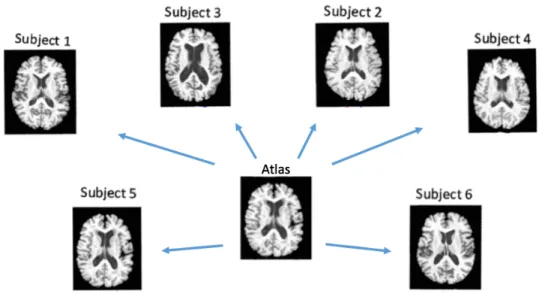
the boxed region in (a). The goal is to align (b) to (c). . . 2 1.2 Example of atlas image and the corresponding subject images. . . 3 1.3 Example of GTPase activations of a cell. Intensities represent the GTPase
activations. Some boundary points are tracked across different time points to extract the corresponding activations and cell movements (velocities).
Refer to Chapter 5 for more details. . . 4
2.1 Framework of the standard image registration. . . 8 2.2 Example of landmark-based registration. The landmarks are superimposed
on (a) source image and (b) target image. The transformed source image and corresponding landmarks are shown in (c). The images are from
(Mod-ersitzki, 2009). . . 9 2.3 Result of Image Analogies: Based on a training set(A, A0)an input image
B can be transformed to B0 which mimics A0 in appearance. The red
circles in (d) show inconsistent regions. . . 10 2.4 Feature matching in the image analogy method: for a pointpin training set
(A, A0), the featurefp forpis extracted from the image patches centered
atp; similarly for a pointq in the input image B and the corresponding sythesizedB0, the featurefqis extracted from the image patches centered
atq. The feature vector concatenates the intensity values for the image patches centered at a pointpin bothAandA0orB andB0. Supposepis the closest point ofq based on the`2 distance of the feature vectors, the
synthesized intensity at pointqinB0is set to the intensity value atpinA0. . . 11
3.1 Flowchart of the proposed method. This method has three components: 1. dictionary learning: learning coupled dictionaries for both training images from different modalities; 2. sparse coding: computing sparse coefficients for the learned dictionaries to reconstruct the source image while at the same time using the same coefficients to transfer the source image to another modality; 3. registration: registering both transferred source image
and target image. . . 20 3.2 Results of estimating a confocal (b) from an SEM image (a) using the
3.3 Prediction errors with respect to differentλvalues for SEM/confocal image.
Theλvalues are tested from 0.05-1.0 with step size 0.05. . . 29 3.4 Results of dictionary learning: the left dictionary is learned from the SEM
and the corresponding right dictionary is learned from the confocal image. . . 30 3.5 Box plot for the registration results of SEM/confocal images on landmark
errors of different methods with three transformation models: rigid, affine and B-spline. The registration methods include: Original Image SSD and Original Image MI, registrations with original images based on SSD and MI metrics respectively; Standard IA SSD and Standard IA MI, registra-tion with standard IA algorithm based on SSD and MI metrics respectively; Proposed IA SSD and Proposed IA MI, registration with the proposed IA algorithm based on SSD and MI metrics respectively. The bottom and top edges of the boxes are the 25th and 75th percentiles, the central red lines
are the medians. . . 30 3.6 Convergence test on SEM/confocal and TEM/confocal images. The
ob-jective function is defined as in Equation (2.11). The maximum iteration number is 100. The patch size for SEM/confocal images and TEM/confocal
images are10×10and15×15respectively. . . 31 3.7 Results of registration for SEM/confocal images using MI similarity
mea-sure with direct registration (first row), standard IA (second row) and the proposed IA method (third row) for (a,d,g) rigid registration (b,e,h) affine registration and (c,f,i) b-spline registration. Some regions are zoomed in to highlight the distances between corresponding fiducials. The images show the compositions of the registered SEM images using the three registration methods (direct registration, standard IA and proposed IA methods) and the registered SEM image based on fiducials respectively. Differences are generally very small indicating that for these images a rigid transformation
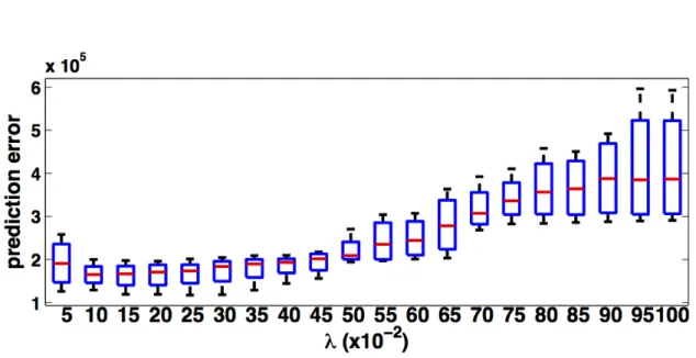
model may already be sufficiently good. . . 33 3.8 Prediction errors for differentλvalues for TEM/confocal image. Theλ
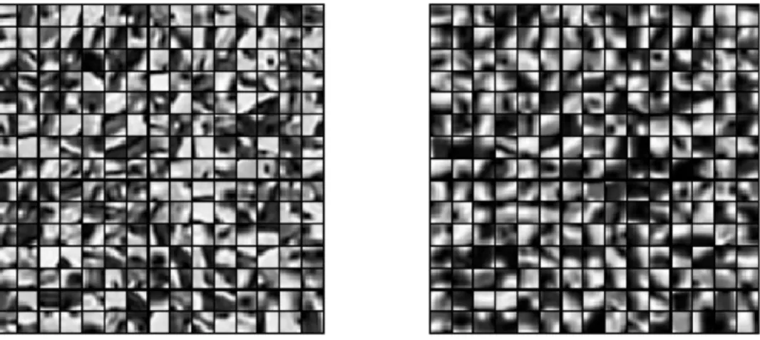
values are tested from 0.05-1.0 with step size 0.05. . . 38 3.9 Results of dictionary learning: the left dictionary is learned from the TEM
and the corresponding right dictionary is learned from the confocal image. . . 39 3.10 Result of estimating the confocal image (b) from the TEM image (a) for the
standard image analogy method (c) and the proposed sparse image analogy
3.11 Results of registration for TEM/confocal images using MI similarity mea-sure with directly registration (first row) and the proposed IA method (sec-ond and third rows) using (a,d,g) rigid registration (b,e,h) affine registration and (c,f,i) b-spline registration. The results are shown in a checkerboard image for comparison. Here, first and second rows show the checkerboard images of the original TEM/confocal images while the third row shows the checkerboard image of the results of the proposed IA method. Differences are generally small, but some improvements can be observed for B-spline registration. The grayscale values of the original TEM image are inverted
for better visualization. . . 40 3.12 Box plot for the registration results of TEM/confocal images for
differ-ent methods. The bottom and top edges of the boxes are 25th and 75th
percentiles, the central red lines indicate the medians. . . 42
4.1 Framework of proposed method. In the training phase, I learn the cou-pled dictionary from training difference images and their corresponding deformations. In the testing phase, I obtain the coefficients for sparse coding of the difference image, and then predict the deformation using the coefficients and the dictionary corresponding to the deformation. Finally applying the deformation to an atlas image results in a registered atlas to a
test image. . . 49 4.2 Illustration of training set and atlas . . . 50 4.3 Illustration of training set generation for experiment in Section 4.4.1. Here,
ti, i= 1, . . . , nare translation vectors which translate the atlas. . . 54
4.4 Translation experiment: Illustration of synthetic (a) atlas image, (b) trans-lated training image, (c) difference image between atlas and transtrans-lated
images. (Intensities in (c) scaled for visualization.) . . . 55 4.5 Deformation prediction results for expriment on synthetic data with random
translations. . . 56 4.6 Image reconstruction results for experiment on synthetic data with random translations 57 4.7 Image reconstruction results with different dictionary size for test image 1 . . . 58 4.8 Illustration of training set generation by shooting with initial momentum . . . 59 4.9 Local deformation experiment (B-Spline) . . . 60 4.10 Results of experiments for B-spline transformation and initial momenta
4.11 Illustration of training set generation by shooting with random initial mo-mentum for the experiment in Section 4.3.3. Here,mi, i = 1, . . . , nare
randomly generated initial momenta. . . 64 4.12 Local deformation experiment: Illustration of synthetic (a) atlas image, (b)
deformed training image, (c) difference image between atlas and deformed images and (d) corresponding initial scalar momentum for experiment in Section 4.3.3. (Note that the intensities in (c) and (d) are scaled for better
visualization.) . . . 64 4.13 Results of local deformation with random initial momenta parametrization
experiment in Section 4.3.3. (a) shows the boxplot of sum of squared differences (SSD) between deformed test images and atlas images with predicted deformation (initial momentum), (b) shows the mean absolute errors (MAE) (in pixels) of each pixel on the deformations for different methods. CDL means standard coupled dictionary learning method, SCDL denotes proposed semi-coupled dictionary learning method, and the num-ber besides the dictionary learning methods indicates the dictionary size
(number of atoms). . . 65 4.14 Illustration of training set and atlas for experiment on OASIA dataset in
Section 4.4.3. Here,mi, i = 1, . . . , nare initial momenta generated by
atlas construction (Singh et al., 2013). . . 66 4.15 Illustration of brain (a) atlas image, (b) subject image, (c) difference image
between atlas and subject images and (d,e) corresponding initial momentum in x and y direction respectively for experiment on OASIA dataset in Section 4.4.3. (Note that the intensities in (c), (d) and (e) are scaled for
better visualization.) . . . 66 4.16 Results of experiment on OASIA dataset in Section 4.4.3. (a) shows the
boxplot of sum of squared differences (SSD) between deformed test im-ages and atlas imim-ages with predicted deformation (initial momentum), (b) shows the mean absolute errors (MAE) (in pixels) of each pixel on the deformations for different methods. CDL means standard coupled dictio-nary learning method, SCDL denotes proposed semi-coupled dictiodictio-nary learning method, and the number besides the dictionary learning methods
indicates the dictionary size(number of items). Image size is128×128. . . 67
5.3 Example of the level set function φt for a boundary Γt. The intensity
values at each pixel indicates the distance to the boundaryΓt. The points
on each circle which are superimposed on φt have the same distance to
the boundary. The numbers on the circles indicate the distances to the boundary with positive values outside the boundary and negative values
inside the boundary. . . 74 5.4 Illustration of boundary tracking. p is the location of a marker on the
boundaryΓt, and the goal is to find the corresponding locationq of the
marker onΓt+1. ∇φtis the gradient direction ofφt. . . 74
5.5 Example of clustering results. . . 77 5.6 Illustration for the parameters in the hypergeometric distribution for the
clusters in activations and velocities. . . 79 5.7 Hypergeometric testing results. The values indicate thep-values for
hyper-geometric testing for the enrichment of clusters based on clustering with GTPase activations and in clusters based on clustering with cell velocities(p-values are corrected using Bonferroni method for multiple tests (Shaffer, 1995)). The null hypothesis is that the clusters with cell velocities are not enriched in clusters with GTPase activations. The left and top blue bars show the distributions of number of data points in different clusters for
activations and velocities respectively. . . 80 5.8 Intersection between different clusters for activations and velocities. The
values indicate the number of intersected data points between different
clusters for activations and velocities. . . 81 5.9 Example of a data point which is represented as linear combination of
dictionary atoms. Blue and red curves indicates protrutions and activations
respectively. The numbers are coefficientsα. . . 82 5.10 Example of prediction results of (a) velocity data for (b) CDL, (c) PCA
and (d) NN methods. The data vectors are reshaped into11×59matrices where 59 is the number of time points of the boundary movement. The
5.11 Example of activations and cell movement patterns. In (a) and (c), the traces of boundary points are superimposed on the cell images, the color of the line indicates timetwhere blue indicatet = 0. The map below each cell image is the activation map corresponding to these boundary points (y axis indicates the index of boundary points and x axis represents time). In (b) and (d), the dictionary atoms are shown to match the corresponding cell movement and activation patterns in (a) and (c) respectively. The displacement plots show the integral of velocities in dictionary atoms, the map below the displacement plot is the corresponding activation map of
the dictionary atoms. . . 88 5.12 Cross correlation for dictionary atoms between rhoA activations and
veloc-ities. X axis indicates different lags between GTPase activations and cell
velocities. . . 89
6.1 Illustration of perfect (left) and imperfect (right) correspondence and their
learned dictionaries . . . 91 6.2 Graphical model for the proposed generative learning framework . . . 100 6.3 D˜ is learned from training images with Gaussian noise (top). Standard
method cannot distinguish corresponding patches and non-corresponding patches while our proposed method can remove non-corresponding patches in the dictionary learning process. The curve (bottom) shows the robustness
with respect toσ1. The vertical green dashed line indicates the learnedσ1. . . 103
6.4 D˜ is learned from training SEM/confocal images with Gaussian noise (top). The curve (bottom) shows the robustness with respect toσ1. The vertical
green dashed line indicates the learnedσ1. . . 104
6.5 TEM/Confocal images . . . 105
A.1 Illustration of search distanceSpi in Equation (A.1).p0 is the location of a marker onΓt, whileqis the corresponding location of the marker onΓt+1.
The goal is to estimate the location ofq. In this example, I usep2 as the
estimation the locationq. Green curve and blue curve represent the cell boundariesΓtandΓt+1at timetandt+ 1respectively;pis the sampled
boundary point;∇φtand ∇φt+1 are the gradient directions of level sets
φt and φt+1 at point prespectively; Sp is the search distance at point p
which is a projection ofDt,t+1(p)onto the unit normal∇φt;θis the angle
between∇φt(pi)and∇φt+1(pi)andcosθcan be computed from the inner
product of ∇φt+1(pi) |∇φt+1(pi)| and
∇φt(pi)
LIST OF ABBREVIATIONS
DL Dictionary Learning
CDL Coupled Dictionary Learning SCDL Semi-coupled Dictionary Learning RCDL Robust Coupled Dictionary Learning
IA Image Analogies
NN Nearest Neighbor
GR Global Regression
SSD Sum of Squared Differences
MI Mutual Information
EM Expectation Maximization
TEM Transmission Electron Microscopy MEF Mouse Embryonic Fibroblast
MR Magnetic Resonance
CHAPTER 1: INTRODUCTION 1.1 Motivations
With the development of new imaging technologies, we can visualize various objects to explore information ranging from molecular structures of cells to tissue of the human body. Different imaging modalities provide distinct information about the objects. For example, in the context of correlative microscopy, which combines different microscopy technologies such as conventional light-, confocal- and electron transmission microscopy (Caplan et al., 2011), protein locations can be revealed through fluorescence microscopy, while protein structures can be observed through electron microscopy (Caplan et al., 2011).
Many image analysis applications require relating the information from different modalities or sources. For example, joint analysis of correlative microscopic images needs registration of images from different modalities as illustrated in Figure 1.1; estimating the deformation of an image with respect to an atlas requires modeling the relationship between deformations and image appearances as illustrated in Figure 1.2; investigating the coordination of GTPase activities and cell protrusions of mouse embryonic fibroblasts (MEFs) requires establishing the spatio-temporal correspondences between GTPase activations and cell movements as illustrated in Figure 1.3.
The similarity between these applications is that they require us tomodel the relationship of data from different spaces.
1.1.1 Multi-modal image registration for correlative microscopy
process of estimating spatial transformations between images (to align them). Registration requires a transformation model and a similarity measure. Direct intensity based similarity measures (such as the sum of squared intensity differences (SSD)) is typically not applicable to multi-modal image registration as image appearances/intensities differ. While a similarity measure such as mutual information (MI) can account for image appearance differences (as MI does not rely on direct image intensity comparisons), it is a very generic measure of image similarity not adapted to a particular application scenario. In general, as images in correlative microscopy differ severely, measuring image similarity is difficult and therefore image registration is challenging. Figure 1.1 shows an example of correlative microscopy.
(a) Confocal Microscopic Image (b) Resampling of Region in (a) (c) TEM Image
Figure 1.1: Example of Correlative Microscopy. (a) is a stained confocal brain slice, where the red box shows a selected region and (b) is a resampled image of the boxed region in (a). The goal is to align (b) to (c).
1.1.2 Deformation estimation from appearances
The deformation estimation problem is challenging as it is difficult to model the relationship between image appearances and deformations. For example, the relation between appearances and deformations could be highly nonlinear.
Figure 1.2: Example of atlas image and the corresponding subject images.
1.1.3 Coordination between GTPase activities and cell movements
Figure 1.3: Example of GTPase activations of a cell. Intensities represent the GTPase activa-tions. Some boundary points are tracked across different time points to extract the corresponding activations and cell movements (velocities). Refer to Chapter 5 for more details.
1.1.4 Coupled dictionary learning
In this dissertation, coupled dictionary learning based approaches are proposed tolearnthese relationships1 from given data. Dictionary learning is a method to learn a basis to represent data (Mairal et al., 2009; Kreutz-Delgado et al., 2003). Typically over-complete dictionaries are used where the number of basis vectors is larger than the dimensionality of the data. Similarly, coupled dictionary learning learns a coupled basis for the data from two coupled spaces. Coupled spaces can for example be the two appearance spaces from two different image modalities. A coupled dictionary can then relate appearances between the two spaces.
1.1.5 Robust coupled dictionary learning
Coupled dictionary learning plays a key role in the previously discussed applications, but presents some challenges: (i) it may fail without sufficient correspondences between the data
1For example, the relationships between appearances of images from different modalities, between appearances and
from different spaces, for example, a low quality image deteriorated by noise in one modality can hardly match a high quality image in another modality. (ii) Usually the data correspondence for two different spaces needs to be obtained before learning the coupled dictionary, for example, by pre-registering training images before dictionary learning. Errors can be introduced during the process of establishing these correspondence.
Thus, a robust dictionary learning method under a probabilistic model is finally introduced in Chapter 6. Instead of directly learning a coupled dictionary from training data, I distinguish between image regions with and without good correspondence in the learning process and update the learned dictionary iteratively.
1.2 Contributions
The main contributions of my work include:
1. a sparse representation and a coupled dictionary learning-based image analogy method to convert and thereby simplify a multi-modal registration problem to a mono-modal one; 2. a general framework for deformation estimation using appearance information based on
coupled dictionary learning;
3. a framework for relating the spatio-temporal patterns between GTPase activations and cell protrusion of mouse embryonic fibroblasts (MEFs) based on coupled dictionary learning; 4. a robust coupled dictionary learning method based on a probabilistic model which
dis-criminates between corresponding and non-corresponding patches automatically.
1.3 Thesis statement
1.4 Outline
The remainder of the document is organized as follows:
CHAPTER 2: BACKGROUND
This chapter provides necessary background and approaches related to this dissertation. Sec-tion 2.1 introduces image registraSec-tion. SecSec-tion 2.2 introduces the standard image analogy method. Section 2.3 provides an introduction to the sparse representation model and its applications in image processing and computer vision. Section 2.4 discusses the dictionary learning method and the numerical solution of the associated learning problem. In Section 2.5, coupled dictionary learning is introduced to capture the relationship between data in two spaces.
2.1 Image registration
Image registration estimates a spatial transformation between a source image and a target image. Letφ(x)denote a transformation that moves a pixel at a locationxin the image to another location,y=φ(x). LetSandT represent the source (moving) image and the target (static) image respectively. The goal of image registration is to estimate the transformationφ(·)for the entire source image that transforms it to match the subject’s image in the sense that, the appearance at a pixely in the deformed source image,S(y) =˜ S(φ−1(y))best matches with the target image, T(y). Figure 2.1 shows the framework for standard image registration (Ibanez et al., 2003; Hill et al., 2001; Maintz and Viergever, 1998). In this framework, image registration is treated as an optimization problem. The interpolator is used to estimate the intensity values of the source image at non-grid locations (Ibanez et al., 2003), while the distance metric d measures the difference between the transformed source image and the target image. The metricdprovides a quantitative measure which can be optimized by the optimizer in the search space defined by the transformation parameters1(Ibanez et al., 2003).
Figure 2.1: Framework of the standard image registration.
There are many image registration methods (Maintz and Viergever, 1998; Zitova and Flusser, 2003). One simple method is landmark-based registration. Here landmarks are a set of points in both source and target images. The idea of landmark-based registration is to estimate a transformation that minimizes the distance between corresponding landmarks in source and target images. Let si = [sxi, syi]denote the position of the ith landmark in the source image andti = [txi, tyi] the
position of the corresponding landmark in the target image, wherei= 1, . . . , n,nis the number of landmarks. Landmark-based registration solves the following minimization problem,
min
φ d(si, ti, φ) = minφ n
X
i=1
kφ(si)−tik22, (2.1)
wheredis the distance between corresponding landmarks, here I use the sum of squared Euclidean distances as an example.
If no landmarks are available, intensity-based registration methods can be applied to the source and target images. Intensity-based methods solve,
min
φ d(S, T, φ) = minφ
X
x∈Ω
kS(φ−1(x))−T(x)k2
(a) source image (b) target image (c) transformed source image
Figure 2.2: Example of landmark-based registration. The landmarks are superimposed on (a) source image and (b) target image. The transformed source image and corresponding landmarks are shown in (c). The images are from (Modersitzki, 2009).
where Ω is the domain of the image, d is the distance which measures the similarity between source and target images. Here I use the sum of squared difference (SSD) as an example. Another commonly used distance measure is mutual information (MI) (Wells et al., 1996).
Which similarity measure to pick for image registration depends on the image pairs to be registered. If they are from the same modality, SSD may be a good choice. For multi-modal approaches more flexible similarity measures such as MI are typically used. However, for image pairs with drastically different appearances such measures may also not be ideal. In this thesis I therefore investigate creating a custom image similarity term via the process of image synthesis which I will discuss next.
2.2 Image analogy
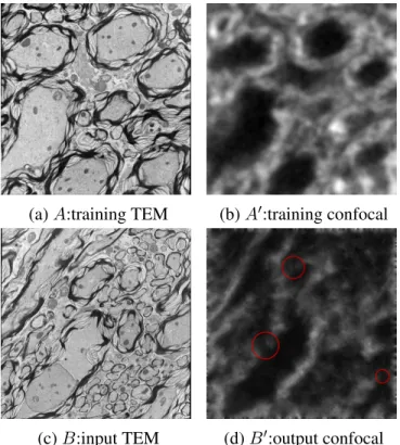
(a)A:training TEM (b)A0:training confocal
(c)B:input TEM (d)B0:output confocal
Figure 2.3: Result of Image Analogies: Based on a training set(A, A0)an input imageB can be transformed toB0 which mimicsA0in appearance. The red circles in (d) show inconsistent regions.
The standard image analogy algorithm achieves the mapping betweenB andB0by looking up best-matching image patches for each image location betweenAandB which then imply the patch appearance forB0from the corresponding patchA0(AandA0 are assumed to be aligned). Examples for image patches are shown in Figure 2.4. These best-matched patches are smoothly combined to generate the overall output imageB0. Figure 2.4 also shows the feature matching between the points inA, A0 andB, B0. The algorithm description is presented in Algorithm 1.
2.2.1 Nearest neighbor search
For multi-modal image registration in Chapter 3, the image analogy approach can be used to transfer a given image from one modality to another using the trained “filter”. Then the multi-modal image registration problem simplifies to a mono-modal one. However, since this method uses a nearest neighbor (NN) search of the image patch centered at each pixel, the resulting images are usually noisy because the`2 norm based NN search does not preserve the local consistency well
Figure 2.4: Feature matching in the image analogy method: for a pointpin training set(A, A0), the featurefpforpis extracted from the image patches centered atp; similarly for a pointqin the input
imageB and the corresponding sythesizedB0, the featurefqis extracted from the image patches
centered atq. The feature vector concatenates the intensity values for the image patches centered at a pointpin bothAandA0 orB andB0. Supposepis the closest point ofqbased on the`2 distance
the number of patches in the NN search, is linearly related to the size of the training images. As a result, NN search is time consuming for large training sets. I introduce a sparse representation model to address these problems in Section 2.3.
Algorithm 1Image Analogies. Input:
Training images: AandA0; Source image: B.
Output:
’Filtered’ sourceB0.
1: Construct Gaussian pyramids forA,A0andB;
2: Generate features forA,A0andB;
3: foreach levellstarting from coarsestdo
4: foreach pixelq ∈Bl0, in scan-line orderdo
5: Find best matching pixelpofqinAlandA0l;
6: Assign the value of pixelpinA0to the value of pixelqinBl0;
7: Record the position ofp.
8: end for
9: end for
10: ReturnBL0 whereLis the finest level.
2.3 Sparse representation
Sparse representation is a powerful model for representing and compressing signals (Wright et al., 2010; Huang et al., 2011b). It represents a signal as a combination (usually linear) of a few fixed basis signals from a typically over-complete dictionary (Bruckstein et al., 2009). It has been successfully applied in many computer vision applications such as for object recognition and classification in (Wright et al., 2009; Huang and Aviyente, 2007; Huang et al., 2011a; Zhang et al., 2012a,b; Fang et al., 2013; Cao et al., 2013a). A dictionary is a collection of basis signals. The number of dictionary elements in an over-complete dictionary exceeds the dimension of the signal space (here the dimension of an image patch). Suppose a dictionaryDis pre-defined. To sparsely represent a signalxthe following optimization problem is solved (Elad, 2010):
ˆ
α =argmin
α
whereαis a sparse vector that explainsxas a linear combination of columns in dictionaryDwith errorandk · k0 indicates the number of non-zero elements in the vectorα. Solving Equation (2.3)
is an NP-hard problem. One possible solution of this problem is based on a relaxation that replaces
k · k0byk · k1, wherek · k1 is the 1-norm of a vector, resulting in the optimization problem,
ˆ
α =argmin
α
kαk1, s.t. kx−Dαk2 ≤. (2.4)
For a suitable choice ofλ, an equivalent problem is given by Equation (2.4)
ˆ
α=argmin
α
kx−Dαk2
2+λkαk1, (2.5)
which is a convex optimization problem that can be solved efficiently (Bruckstein et al., 2009; Boyd et al., 2010; Mairal et al., 2009). The optimization problem Equation (2.5) is asparse coding
problem which finds the sparse codesαto representx. Based on the sparse representation model, an over-complete basis, i.e. a dictionary, can be learned for the reconstruction of data in some space. 2.4 Dictionary learning
Dictionary learning plays a key role in many applications using sparse models. As a result, many dictionary learning methods have been introduced in recent literature (Aharon et al., 2006; Yang et al., 2010; Mairal et al., 2008; Monaci et al., 2007). In (Aharon et al., 2006), a dictionary is learned for image denoising, while in (Mairal et al., 2008), supervised dictionary learning is performed for classification and recognition tasks. Given sets of training dataxi, the goal is to
estimate the dictionaryDas well as the coefficientsαifor the sparse coding problem,
{αˆi,Dˆ}=argmin αi,D
N
X
i=1
kxi−Dαik22+λkαik1, (2.6)
whereN is the number of training datasets, and λis the parameter to control the sparsity ofαi.
to approximatexi. To avoidDbeing arbitrarily large, each column ofDis normalized to have`2
norm less than or equal to one, i.e. dT
kdk≤1, fork = 1, ..., p,andD={d1, d2, ..., dq} ∈Rp×q.
2.4.1 Data preprocessing
Let X be the data matrix X = {x1, x2, . . . , xn} ∈ Rp×n, each column in X represents a
data vector, while each row ofX represents a feature. UsuallyX requires preprocessing before dictionary learning. There are three commonly used data preprocessing methods.
Mean subtraction: Here, for each feature in the data matrix its mean across all data points is subtracted. The geometric interpretation of mean subtraction is centering the data around the origin for every feature dimension.
Feature Scaling: Here, each feature in the data matrix is divided by its standard deviation across all data points after mean subtraction. It is usually applied to data where each feature has a different scale but equal importance to the learning algorithm. For image patches, it is not necessary to apply feature scaling because the relative scales of pixels are approximately equal (usually between 0 and 255).
Normalization: Here, each data vector is normalized to unit norm by division with its`2 norm.
Note that it is not necessary to apply all the preprocessing steps to the data. Choosing appropriate data preprocessing methods is based on the applications. I will give an example in Section 3.3.3. 2.4.2 Numerical solution
The optimization problem in Equation (2.6) is non-convex (bilinear inDandαi). The standard
approach (Elad, 2010) is alternating minimization, i.e., solving forαi keepingDfixed and vice
versa. By fixingD, we first solve the sparse coding problems,
ˆ
αi =argmin αi
N
X
i
kxi−Dαik22+λkαik1. (2.7)
algorithm minimizes Equation (2.7) with respect to one component ofαin one step, keeping all other components constant. This step is repeated until convergence.
Algorithm 2Coordinate Descent for Sparse Coding Input: α = 0, λ >0, β =DTx
Output: α
whilenot convergeddo 1. α˜ =Sλ(β)1;
2. j =argmaxi|αi−α˜i|, whereiis the index of the component inαandα;˜
3. αki+1 =αik, i =6 j, andαkj+1 = ˜αj;
4. βk+1 = βk − |αk
j −α˜j|(DTD)j, and βjk+1 = βjk, where (DTD)j is thejth column of
(DTD). end while
After solving Equation (2.7), I can fix αi and then update D. Now the optimization of
Equation (2.6) can be changed to
ˆ
D=argmin
D N
X
i=1
kxi−Dαik22. (2.8)
The closed-form solution of Equation (2.8) is as follows,
D= (
N
X
i=1
xiαTi )( N
X
i=1
αiαTi )
−1
. (2.9)
The columns are normalized according to
dj =dj/max(kdjk2,1), j = 1, ..., m, (2.10)
whereD={d1, d2, ...dm} ∈ Rnxm.I iterate the optimization with respect toDandαi to
conver-gence.
2.5 Coupled dictionary learning
Coupled dictionary learning is a method to learn a joint basis for compact representation of the data from two spaces (Yang et al., 2012a,b). In (Monaci et al., 2007), a coupled dictionary
2S
is learned from audio-visual data. A coupled dictionary which has two parts corresponding to different modalities, can be also applied to super-resolution (Yang et al., 2010) and multi-modal image registration (Cao et al., 2012).
2.5.1 Standard coupled dictionary learning (CDL)
Given sets of corresponding training pairs{x(1)i , x(2)i }, the coupled dictionary learning problem can be formulated as
{D,ˆ˜ αˆ}=argmin
˜ D,α N X i=1 1 2kx˜i−
˜
Dαik22+λkαik1, (2.11)
whereD˜ = [D(1), D(2)]T stacks two different dictionaries andx˜i = [x
(1)
i , x
(2)
i ]T, is the corresponding
stacked training data from two different spaces. Note that there is only one set of coefficientsαi per
datum, which enforces correspondence of the dictionaries between the two spaces. The numerical solution for standard CDL is the same as the solution mentioned in Section 2.4.2.
2.5.2 Semi-coupled dictionary learning (SCDL)
In standard coupled dictionary learning, using only one set of coefficients imposes the strong assumption that coefficients of the representation of the two spaces are equal. However, this strong assumption sometimes does not hold. To relax this assumption, a semi-coupled dictionary learning is proposed in (Wang et al., 2012),
{Dˆ(1),Dˆ(2),{αˆ(1)i },{αˆ(2)i },Wˆ}= argmin
D(1),D(2),{α(1) i },{α
(2) i },W
N
X
i=1
1 2kx
(1)
i −D
(1)α(1)
i k
2 2+
1 2kx
(2)
i −D
(2)α(2)
i k
2
2+λ1kα (1)
i k1+λ2kα (2)
i k1+γ1kα (2)
i −W α
(1)
i k
2
2+γ2kWk2F,
(2.12)
whereλ1,λ2,γ1,γ2 are regularization parameters. Distinct from CDL,W is a matrix to define a
mapping between the coefficients in two spaces. Equation (2.11) is a special case of Equation (2.12) whenW equals the identity andα(1)equalsα(2). Unlike for CDL the columns of the dictionaries
normalization is beneficial to jointly compute a basis for appearance differences and deformations. Equation (2.12) is not convex with respect toD(1),D(2),α(1),α(2),W jointly, however, it is convex
with respect to each of them when others are fixed. 2.5.3 Numerical solution
Equation (2.12) can be solved by an iterative algorithm updatingD(1),D(2),W alternatingly. I
initializeW as identity matrix andD(1) ={d(1)1 , . . . , d(1)m }andD(2) ={d(2)1 , . . . , d (2)
m }asmrandom
x(1)i andx(2)i pairs. WithW,D(1),D(2) fixed, I solve the following sparse coding problems with respect toα(1)i andα(2)i ,
min
α(1)i N
X
i=1
1 2kx
(1)
i −D
(1)
α(1)i k22+γ1kα(2)i −Wαˆ
(1)
i k
2
2+λ1kα(1)i k1,
min
α(2)i N
X
i=1
1 2kx
(2)
i −D
(2)
α(2)i k22+γ1kαˆ(2)i −W α
(1)
i k
2
2+λ2kα(2)i k1,
(2.13)
where αˆ(1)i and αˆ(2)i are results obtained from the previous iteration. Equation (2.13) are lasso problems which can be solved by Algorithm 2 or other existing `1 solvers such as coordinate
descent (Friedman et al., 2007), FISTA (Beck and Teboulle, 2009) and LARS (Efron et al., 2004). By fixingW,α(1)i andα(2)i , based on Equation (2.11), I updateD(1)andD(2)by solving
min
D(1),D(2)
N
X
i=1
1 2kx
(1)
i −D
(1)α(1)
i k
2 2 +
1 2kx
(2)
i −D
(2)α(2)
i k
2 2,
s.t.kd(1)j k2 ≤1, kd (2)
j k ≤1, j = 1, . . . , m,
(2.14)
whereD(1) ={d(1)1 , . . . , dm(1)}, D(2) ={d(2)1 , . . . , d (2)
m }. Equation (2.14) can be decoupled into two
problems, thus the least-squares solutions for the dictionaries are obtained by computing
D(1) = (
N
X
i=1
x(1)i (α(1)i )T)(
N
X
i=1
α(1)i (α(1)i )T)−1,
D(2) = (
N
X
i=1
x(2)i (α(2)i )T)(
N
X
i=1
α(2)i (α(2)i )T)−1.
Projection onto the`2 ball is achieved by
d(1)j =d(1)j /max(kd(1)j k2,1), d (2)
j =d
(2)
j /max(kd
(2)
j k2,1).
Finally by fixingD(1),D(2),α(1)i andα(2)i , I can updateW by solving,
min
W N
X
i=1
γ1kα (2)
i −W α
(1)
i k
2
w +γ2kWk2F. (2.16)
The closed-form solution of Equation (2.16) is:
W = (
N
X
i=1
γ1α (2) i (α (1) i ) T )( N X i=1
γ1α (1)
i (α
(1)
i ) T
+γ2I)−1.
2.6 Conclusion
CHAPTER 3: COUPLED DICTIONARY LEARNING FOR MULTI-MODAL REGISTRA-TION
Multi-modal registration is a crucial step to analyze images from different modalities such as correlative microscopy images (Lemoine et al., 1994; Caplan et al., 2011). The goal of image registration is to compute the spatial alignment between images by maximizing the similarity between images in the space of admissible transformations. Here, defining image similarity is challenging as images may have strikingly different appearances. Hence, standard image similarity measures may not apply. In this chapter, I propose a method to transform the appearance of an image from one modality to another. By transforming the appearance of the image, a multi-modal registration problem can be simplified to a mono-modal one. The appearance transformation can be realized by image analogy1. The proposed image analogy method is based on coupled dictionary learning. The flowchart of my method is shown in Figure 3.1.
3.1 Introduction
Correlative microscopy integrates different microscopy technologies including conventional light-, confocal- and electron transmission microscopy (Caplan et al., 2011) for the improved examination of biological specimens. For example, fluorescent markers can be used to highlight regions of interest combined with an electron-microscopy image to provide high-resolution structural information of the regions. To allow such joint analysis requires the registration of multi-modal microscopy images. This is a challenging problem due to (large) appearance differences between the image modalities.
Image registration which was introduced in Section 2.1 is an essential part of many image analysis approaches. The registration of correlative microscopic images is very challenging: images should carry distinct information to combine, for example, knowledge about protein locations (using fluorescence microscopy) and high-resolution structural data (using electron microscopy). However, this precludes the use of simple alignment measures such as the sum of squared intensity differences because intensity patterns do not correspond well or a multi-channel image has to be registered to a gray-valued image.
A solution for the registration of correlative microscopy images is to perform landmark-based alignment (Section 2.1), which can be greatly simplified by adding fiducial markers (Fronczek et al., 2011). Fiducial markers cannot easily be added to some specimens, hence an alternative intensity-based method is needed. This can be accomplished in some cases by appropriate image filtering. This filtering is designed to only preserve information which is indicative of the desired transformation, to suppress spurious image information, or to use knowledge about the image formation process to convert an image from one modality to another. For example, multichannel microscopy images of cells can be registered by registering their cell segmentations (Yang et al., 2008). However, such image-based approaches are highly application-specific and difficult to devise for the non-expert. If the images are structurally similar (for example when aligning EM images of different resolutions (Kaynig et al., 2007), standard feature point detectors can be used.
alignment of sets of training images which can easily be accomplished by a domain specialist who does not need to be an expert in image registration.
Arguably, transforming image appearance is not necessary if using an image similarity measure which is invariant to the observed appearance differences. In medical imaging, mutual information (MI) (Wells et al., 1996) is the similarity measure of choice for multi-modal image registration. I show for two correlative microscopy example problems that MI registration is indeed beneficial, but that registration results can be improved by combining MI with an image analogies approach. To obtain a method with better generalizability than standard image analogies (Hertzmann et al., 2001) I devise an image analogies method using ideas from sparse coding (Bruckstein et al., 2009), where corresponding image patches are represented by a learned basis (a dictionary). Dictionary elements capture correspondences between image patches from different modalities and therefore allow to transform one modality to another modality.
This chapter is organized as follows: First, I briefly introduce some related work in Section 3.2. Section 3.3 describes the proposed method for multi-modal registration. Image registration results are shown and discussed in Section 3.4. The chapter concludes with a summary of results and an outlook on future work in Section 3.5.
3.2 Related work
3.2.1 Multi-modal image registration for correlative microscopy
Since correlative microscopy combines different microscopy modalities, resolution differences between images are common. This poses challenges with respect to finding corresponding regions in the images. If the images are structurally similar (for example when aligning EM images of different resolutions (Kaynig et al., 2007)), standard feature point detectors can be used.
and Navab, 2010). The motivation of the proposed method is similar to Wachinger’s approach, i.e. transform the modality of one image to another, but I use an image analogy approach to achieve this goal thereby allowing for the reconstruction of a microscopy image in the appearance space of another.
3.2.2 Image synthesis
Image synthesis is a process to create new images from given images or image descrip-tions (Fisher et al., 1996). Image analogy, first introduced in (Hertzmann et al., 2001), is an image synthesis method which has been used widely in texture synthesis. In (Prince et al., 1995; Fis-chl et al., 2004), the authors proposed a method to synthesize magnetic resonance (MR) images. In (Roy et al., 2011), the authors introduced a compressed sensing based approach for MR tissue contrast synthesis, however, the dictionary is generated by random selection from the training data. In (van Tulder and de Bruijne, 2015), the authors proposed a restricted Boltzmann machines (RBM) based approach to synthesize MRI images for classification, however, the authors only reported the accuracy and whether the method improved the image synthesis results (how similar a synthesized image is compared to the original image is unknown). In (Iglesias et al., 2013), the authors applied a simplified image analogy method to demonstrate the benefits of synthesis in registration and segmentation for MRI images.
For multi-modal image registration, an image synthesis method can be used to transfer a given image from one modality to another. Then the multi-modal image registration problem simplifies to a mono-modal one. I use image analogy for modality transformation in this chapter because image analogy is a simple and straightforward image synthesis method and many other applications are based on this method such as image super-resolution (Freeman et al., 2002) and image completion (Drori et al., 2003).
However, since this method uses a nearest neighbor (NN) search of the image patch centered at each pixel, the resulting images are usually noisy because the`2 norm based NN search does not
among neighboring pixels, but an effective solution is still missing. I introduce a dictionary learning based image analogy method to address this problem in Section 3.3.1.
The contribution of this chapter is two-fold.
• I introduce a sparse representation model for image analogy with the goal of improving the image analogy accuracy.
• I simplify multi-modal image registration by using the image analogy approach to convert the registration problem to a mono-modal registration problem.
3.3 Method
The standard coupled dictionary learning (CDL) approach has been introduced in Section 2.5. This section introduces the CDL based image analogy method.
3.3.1 CDL for image analogies
For the registration of correlative microscopy images, given two training imagesAandA0 from different modalities, imageB can be transformed to the other modality by synthesizingB0using the image analogy approach. Consider the sparse dictionary-based image denoising/reconstruction, u, given by minimizing
E(u,{αi}) =
γ
2kLu−fk
2 2+
1 2
N
X
i=1
kRiu−DαikV2 +λkαik1, (3.1)
wheref is the given (potentially noisy) image,Dis the dictionary,{αi}are the patch coefficients,
Ri selects theith patch from the image reconstructionu,γ,λ >0are balancing constants,Lis a
linear operator (e.g., describing a convolution), and the norm is defined askxk2
v =xTV x, where
image. Formulation Equation (3.1) can be extended to image analogies by minimizing
E(u(1), u(2),{αi}) = γ 2kL
(1)
u(1)−f(1)k22
+1 2
N
X
i=1
kRi
u(1) u(2) − D(1) D(2) αik
2
V +λkαik1,
(3.2)
where I have corresponding dictionaries {D(1), D(2)}and only one imagef(1)is given and I am
seeking a reconstruction of a denoised version off(1),u(1), as well as the corresponding analogous denoised imageu(2)(without the knowledge off(2)). Note that there is only one set of coefficients αi per patch, which indirectly relates the two reconstructions. The problem is convex (for given
D(i)) which allows to compute a globally optimal solution.
Patch-based (non-sparse) denoising has also been proposed for the denoising of fluorescence microscopy images (Boulanger et al., 2010). A conceptually similar approach using sparse coding and image patch transfer has been proposed to relate different magnetic resonance images in (Roy et al., 2011). However, this approach does not address dictionary learning or spatial consistency considered in the sparse coding stage. My approach addresses both and learns the dictionariesD(1) andD(2) explicitly.
3.3.2 Numerical solution
To simplify the optimization process of Equation (3.2), I apply an alternating optimization approach (Elad, 2010) which initializesu(1) = f(1) and u(2) = D(2)αat the beginning, and then
computes the optimal α (the dictionaries D(1) and D(2) are assumed known here). Thus the
minimization problem breaks into many smaller subparts, for each subproblem I have,
ˆ
α= arg min
α
1 2kRiu
(1)−D(1)α
ik22+λkαik1, i∈1, ...N . (3.3)
GivenA=D(1),x= α
i andb =Riu(1), then Equation (3.3) can be rewritten in the general
form
ˆ
x= arg min
x
1
2kb−Axk
2
2+λkxk1. (3.4)
The coordinate descent algorithm to solve Equation (3.4) is described in Algorithm 2. This algorithm minimizes Equation (3.4) with respect to one component ofxin one step, keeping all other components constant. This step is repeated until convergence.
After solving Equation (3.3), I can fix α and then update u(1). Now the optimization of Equation (3.2) can be changed to
ˆ
u(1) = arg min
u(1) γ 2ku
(1)−f(1)k2 2+
N
X
i=1
1 2kRiu
(1)−D(1)α
ik22. (3.5)
The closed-form solution of Equation (3.5) is as follows2,
ˆ
u(1) = (γI+
N
X
i=1
RTi Ri)−1(γf(1)+ N
X
i=1
RTi D(1)αi). (3.6)
I iterate the optimization with respect tou(1)andαto convergence. Thenu(2) = (PN
i R T
i Ri)−1D(2)α.ˆ
3.3.3 Intensity normalization
The image analogy approach may not be able to achieve a perfect prediction because: (i) image intensities are normalized and hence the original dynamic range of the images is not preserved and (ii) image contrast may be lost as the reconstruction is based on the weighted averaging of patches. To reduce the intensity distribution discrepancy between the predicted image and original image, in this method, I apply intensity normalization (normalize the different dynamic ranges of different images to the same scale for example[0,1]) to the training images before dictionary learning, and also to the image analogy results.
3.3.4 Use in multi-modal image registration
For image registration, I (i) reconstruct the “missing” analogous image and (ii) consistently denoise the given image to be registered with (Elad and Aharon, 2006). By denoising the target image using the learned dictionary for the target image from the joint dictionary learning step I obtain two consistently denoised images: the denoised target image and the predicted source image. The image registration is applied to the analogous image and the target image. I consider rigid followed by affine and B-spline registrations in this chapter and use the implementation of the Elastix toolbox (Klein et al., 2010; Ibanez et al., 2003). As similarity measures I use sum of squared differences (SSD) and mutual information (MI). A standard gradient descent is used for optimization. For B-spline registration, I use displacement magnitude regularization which penalizeskT(x)−xk2, whereT(x)is the transformation of coordinatexin an image (Klein et al.,
2010). This is justified as I do not expect large deformations between the images as they represent the same structure. Hence, small displacements are expected, which are favored by this form of regularization.
3.4 Results 3.4.1 Data
I use both 2D correlative SEM/confocal images with fiducials and TEM/confocal images of mouse brains for the experiment. All experiments are performed on a Dell OptiPlex 980 computer with an Intel Core i7 860 2.9GHz CPU. The data description is shown in Table 3.1.
Table 3.1: Data Description Data Types
SEM/confocal TEM/confocal
Number of datasets 8 6
Fiducial 100nmgold none
3.4.2 Registration of SEM/confocal images (with fiducials) 3.4.2.1 Data preparation
The confocal images are denoised by the sparse representation based denoising method (Elad, 2010). I use a landmark based registration on the fiducials to obtain the gold standard alignment results. The image size is about400×400pixels.
3.4.2.2 Image analogy (IA) results
(a) SEM Image (b) Confocal Image (c) Standard IA (d) Proposed IA
Figure 3.2: Results of estimating a confocal (b) from an SEM image (a) using the standard IA (c) and the proposed IA method (d).
Figure 3.4: Results of dictionary learning: the left dictionary is learned from the SEM and the corresponding right dictionary is learned from the confocal image.
Table 3.2: Prediction results for SEM/confocal images. Prediction is based on the proposed IA and standard IA methods. I used sum of squared prediction residuals (SSR) to evaluate the prediction results. The p-value is computed using a paired t-test.
Method mean std p-value
Proposed IA 1.52×10⁵ 5.79×10⁴
0.0002 Standard IA 2.83×10⁵ 7.11×10⁴
3.4.2.3 Image registration results
I resampled the estimated confocal images with up to±600 nm(15 pixels) in translation in the x and y directions (at steps of 5 pixel) and±15◦in rotation (at steps of 5 degree) with respect to the gold standard alignment. Then I registered the resampled estimated confocal images to the corresponding original confocal images. The goal of this experiment is to test the ability of the proposed methods to recover from misalignments by translating and rotating the pre-aligned image within a practically reasonable range. Such a rough initial automatic alignment can for example be achieved by image correlation. The image registration results based on both image analogy methods are compared to registration results using original images using both SSD and MI as similarity measures3. Table 3.4 summarizes the registration results on translation and rotation errors based on the rigid transformation model for each image pair over all these experiments. The results are reported as physical distances instead of pixels. I also perform registrations using affine and B-spline transformation models. These registrations are initialized with the result from the rigid registration. Figure 3.5 shows the box plot for all the registration results. The proposed method achieves the best registration results for all three transformation models compared with directly registering the multi-modal images and the standard image analogy method. However, the proposed methods increase the registration results little with more flexible transformation models i.e. affine and b-spline models.
(a) (b) (c)
(d) (e) (f)
(g) (h) (i)
Table 3.3: CPU time (in seconds) for SEM/confocal images. The p-value is computed using a paired t-test.
Method mean std p-value
Proposed IA 82.2 6.7
0.00006 Standard IA 407.3 10.1
3.4.2.4 Hypothesis test on registration results
In order to check whether the registration results from different methods are statistically different from each other, I use hypothesis testing (Weiss and Weiss, 2012). I assume the registration results (rotations and translations) are independent and normally distributed random variables with meansµi and variancesσ2i. For the results from 2 different methods, the null hypothesis (H0) is
µ1 = µ2, and the alternative hypothesis (H1) is µ1 ≤ µ2. I apply the one-sided paired sample
Table 3.4: SEM/confocal rigid registration errors on translation (t) and rotation (r)(t =p t2
x+t2y
wheretx and ty are translation errors in x and y directions respectively;tis in nm; pixel size is
40nm;ris in degree.) Here, the registration methods include: Original Image SSD and Original Image MI, registrations with original images based on SSD and MI metrics respectively; Standard IA SSD and Standard IA MI, registration with standard IA algorithm based on SSD and MI metrics respectively; Proposed IA SSD and Proposed IA MI, registration with the proposed IA algorithm based on SSD and MI metrics respectively.
rmean rmedian rstd tmean tmedian tstd
Proposed IA SSD 0.357 0.255 0.226 92.457 91.940 56.178 Proposed IA MI 0.239 0.227 0.077 83.299 81.526 54.310 Standard IA SSD 0.377 0.319 0.215 178.782 104.362 162.266
Table 3.6: Hypothesis test results (p-values) with multiple testing correction results (FDR corrected p-values in parentheses) for registration results measured via landmark errors for SEM/confocal images. I use a one-sided paired t-test. Comparison of different registration models (rigid, affine, B-spline) within the same image types (original image, standard IA, proposed IA). Results are not statistically significantly better after correcting for multiple comparisons with FDR.)
Rigid/Affine Rigid/B-spline Affine/B-spline Original Image SSD 0.7918 (0.8908) 0.3974 (0.6596) 0.1631 (0.5873) MI 0.6122 (0.7952) 0.3902 (0.6596) 0.3635 (0.6596) Standard IA SSD 0.9181 (0.9371) 0.1593 (0.5873) 0.0726 (0.5873) MI 0.5043 (0.7564) 0.6185 (0.7952) 0.7459 (0.8908) Proposed IA SSD 0.9371 (0.9371) 0.3742 (0.6596) 0.0448 (0.5873) MI 0.4031 (0.6596) 0.1616 (0.5873) 0.2726 (0.6596)
3.4.2.5 Discussion
From Figure 3.5, the improvement of registration results within an individual registration model from rigid registration to affine and B-spline registrations are not significant due to the fact that both SEM/confocal images are acquired from the same piece of tissue section. The rigid transformation model can capture the deformation well enough, though small improvements can visually be observed using more flexible transformation models as illustrated in the composition images between the registered SEM images using three registration methods (direct registration and the two IA methods) and the registered SEM images based on fiducials of Figure 3.7. The proposed method can achieve the best results for all the three registration models. See also Table 3.6. The results show that the similarity measures matters (my method is best) for the registration. However, the different transformation models do not matter much for this experiment.
3.4.3 Registration of TEM/confocal images (without fiducials) 3.4.3.1 Data preparation