Multiple Imputation of missing values in exploratory factor analysis
of multidimensional scales: estimating latent trait scores
Urbano Lorenzo-Seva1* y Joost R. Van Ginkel2
1 CRAMC (Research Center for Behavior Assessment); Department of Psychology; Universitat Rovira i Virgili (Tarragona, Spain) 2 Leiden University (Leiden, The Netherlands)
Título: Imputación múltiple de valores perdidos en el análisis factorial
ex-ploratorio de escalas multidimensionales: estimación de las puntuaciones de rasgos latentes.
Resumen: Los investigadores con frecuencia se enfrentan a la difícil tarea
de analizar las escalas en las que algunos de los participantes no han res-pondido a todos los ítems. En este artículo nos centramos en el análisis factorial exploratorio de escalas multidimensionales (es decir, escalas que constan de varias de subescalas), donde cada subescala se compone de una serie de ítems de tipo Likert, y el objetivo del análisis es estimar las puntua-ciones de los participantes en los rasgos latentes correspondientes. En este contexto, se propone un nuevo enfoque para hacer frente a las respuestas faltantes que se basa en (1) la imputación múltiple de las respuestas faltan-tes y (2) la rotación simultánea de las muestras de datos imputados. Se ha aplicado el método en una muestra de datos reales en que las respuestas que faltantes fueron introducidas artificialmente siguiendo un patrón real de respuestas faltantes, y un estudio de simulación basado en conjuntos de datos artificiales. Los resultados muestran que nuestro enfoque (en concre-to, Hot-Deck de imputación múltiple seguido de rotación Consensus Promin) es capaz de calcular correctamente la puntuación factorial estima-da incluso para los participantes que tienen valores perdidos.
Palabras clave: Valores perdidos; Imputación Hot-Deck; Imputación
Pre-dictive mean matching; Imputación múltiple; Consensus Rotation; Puntuaciones factoriales; Análisis factorial exploratorio.
Abstract: Researchers frequently have to analyze scales in which some
participants have failed to respond to some items. In this paper we focus on the exploratory factor analysis of multidimensional scales (i.e., scales that consist of a number of subscales) where each subscale is made up of a number of Likert-type items, and the aim of the analysis is to estimate par-ticipants’ scores on the corresponding latent traits. We propose a new ap-proach to deal with missing responses in such a situation that is based on (1) multiple imputation of non-responses and (2) simultaneous rotation of the imputed datasets. We applied the approach in a real dataset where missing responses were artificially introduced following a real pattern of non-responses, and a simulation study based on artificial datasets. The re-sults show that our approach (specifically, Hot-Deck multiple imputation followed of Consensus Promin rotation) was able to successfully compute factor score estimates even for participants that have missing data.
Key words: Missing data; Hot-Deck imputation;Predictive mean
match-ing imputation; Multiple imputation; Consensus Rotation; Factor scores; Exploratory factor analysis.
1*
Introduction
The ultimate aim of psychological testing is to estimate the score of a person in one or more latent psychological varia-bles (known as latent traits). The estimate is based on a per-son’s answers to a set of items (i.e. a psychological test): each item in the test helps the person to report a particular facet of his/her own personality or how (s)he would react or feel in a particular situation. Frequently, these items are Likert-type items: responses to items are based on a binary or a graded format. With this aim (i.e., to estimate factor scores from responses to Likert-type items), psychological test data obtained in a large sample is typically analyzed using explora-tory factor analysis (EFA). However, as responses to Likert-type items cannot be regarded as continuous-unbounded variables, typical linear factor analysis is inappropriate in this situation. An alternative to linear factor analysis is the non-linear Underlying Variable Approach (UVA; see, for exam-ple, Mislevy, 1986; Moustaki, Joreskog, & Mavridis, 2004).
The UVA uses a two-level approach: on the first level, it is assumed that the observed item response arises as a result of a categorization of an underlying response variable; on the
* Dirección para correspondencia [Correspondence address]:
Urbano Lorenzo-Seva, Departament de Psicologia; Universitat Rovira i Virgili; Carretera de Valls s/n; 43007, Tarragona (Spain).
E-mail: [email protected]
second level, it is assumed that the linear model holds for these underlying responses. Parameters are estimated from the bivariate tetrachoric/polychoric tables between pairs of item scores. The simplest and most usual approach is known as the heuristic solution (Bock & Aitkin, 1981): item thresholds are estimated from the marginals of the table, and the tet-rachoric/polychoric correlations are estimated from the joint frequency cells. Then, the usual factor analysis of the poly-choric correlation matrix provides estimates of item loadings and residual variances. Once the estimates have been ob-tained, they can be reparameterized so that the model is re-ported in the most usual (multidimensional) Item Response Theory (IRT) form (see, for example, Ferrando & Lorenzo-Seva, 2013). Finally, factor scores on the latent variables can be estimated. One popular approach is to compute expected a posteriori (EAP) estimators, which have good properties that other estimators do not usually have (Muraki & Engel-hard, 1985). It must be noted that, in order to compute these factor-score estimates for a particular individual in the sam-ple, (s)he must have provided an answer to each item in the psychological test. However, a typical difficulty when
analyz-ing the responses of a sample of participants is missing data:
some respondents fail to respond to some items (item nonre-sponse).
with low lexical abilities may not respond to an item that in-cludes a complex word. Rubin (1976) formalized the three mechanisms that underlie the missing data process: (a) miss-ing completely at random (MCAR), (b) missmiss-ing at random (MAR), and (c) missing not at random (MNAR). The MCAR values occur when the probability that a particular value is missing in the data set is independent of all other (observed and non-observed) variables. As a consequence, the missing values occur randomly for all variables in the data set. The MAR values occur when the probability that a value is miss-ing depends on the observed variables in the data set, but not on the unobserved variables. The MNAR values occur when the probability that a value is missing depends on un-observed variables.
Even if the problem of item nonresponse is as old as psychological testing, it can still be an obstacle in studies nowadays. For example, in a recent study on marital happi-ness, Johnson and Young (2011) observed that the percent-age of missing responses was highest for questions about sexual behavior (23%) and total household income (19% to 27%). Schlomer, Bauman and Card (2010) recently studied how researchers currently cope with missing responses in applied research (Vol. 55 of the Journal of Counseling Psychology, 2008), and concluded that, despite the prevalence of missing data and the existence of recommendations for taking these data into account, this journal had not yet done so. Nowa-days, research journals are publishing papers on best practic-es and recommendations about missing rpractic-esponspractic-es (see, for example, Cuesta, Fonseca, Vallejo, & Muñiz,, 2013, Graham, 2009, Kleinke, Stemmler, Reinecke, & Lösel, , 2011).
In order to cope with missing responses, incomplete re-sponse patterns are often deleted from the sample (listwise deletion or pairwise deletion). Even though this is easy to do, deleting cases with missing responses could lead to bias in the parameter estimates of the factor model (for example, loading values). In addition, because some responses are missing, the estimated score on the latent variable cannot be computed for those individuals with incomplete response patterns. One of the techniques recommended for handling
item nonresponse is imputation: the missing values are filled in
so that a complete data set is created and then analyzed with traditional methods of analysis. However, single imputation methods are considered outdated (see for example, Schafer & Graham, 2002). While single imputation can lead to ap-proximately unbiased point estimates, estimated standard er-rors are systematically underestimated (Rässler, Rubin, & Zell, 2013).
A more elaborate approach to filling in missing responses
is the multiple imputation (MI) method (Rubin, 1978): instead
of creating a single complete data set, a number of copies are created by imputation. Then, each copy of data is analyzed independently, and the final outcome is obtained as a com-bination of the outcomes obtained in the copies of data. One advantage of MI is that the final standard errors of these pa-rameter estimates are based on both (a) the standard errors of the analysis of each data set and (b) the dispersion of
pa-rameter estimates across data sets. As MI accounts for the random fluctuations between each imputation, it provides accurate standard errors and therefore accurate inferential conclusions. If MI is a general method, it can be applied us-ing different techniques (i.e., the complete copies of data can be generated using different approaches). Nowadays, the use of MI is quite popular in applied research in psychology: a Google search for the terms psychology “multiple imputation” produces about 131,000 hits.
Within the framework of IRT, missing values are fre-quently treated as if they were the result of an incomplete testing design (i.e., subsets of items administered to different respondents) (see, for example, DeMars, 2003). The resulting incomplete data can be analyzed with IRT models and esti-mates of latent abilities. However, as Huisman and Molenaar (2001) point out, this strategy for handling item-nonresponse cannot be used in every situation. When this approach is not feasible, imputation of missing data appears as an advisable alternative. Imputation of missing data in IRT has been stud-ied in the context of unidimensional models (Ayala, Plake, & Impara, 2001; DeMars, 2003; Finch, 2008, 2011; Huisman & Molenaar, 2001; Sijtsma & Van der Ark, 2003). Recently, Wolkowitz and Skorupski (2013) proposed a single imputa-tion approach intended to estimate statistical properties of items but not factor scores. Finally, no research has yet been undertaken in the framework of multidimensional IRT.
MI has already been proposed in the context of confirm-atory factor analysis, and can be computed using, for exam-ple, Mplus (Muthén & Muthén, 1998-2011). In this context, the copies of data created using MI are analyzed inde-pendently but with one restriction: they share the same hy-pothesis for the factor solution in the population. The fact that all the copies of data share the same hypothesis means that the outcomes of the copies of data are comparable, and may consequently be combined to produce one final out-come. However, Mplus does not allow MI to be computed in the the context of EFA: as there is no hypothesis of the factor solution in the population (because of the exploratory nature of the analysis), the outcomes obtained in different copies of data are not necessarily comparable. This means that the EFA outcomes that are produced for each data copy cannot be directly combined to produce one final outcome. This last difficulty seems to indicate that MI cannot be used in EFA.
Procedure to obtain estimates of latent trait
scores for ordinal data when data is missing
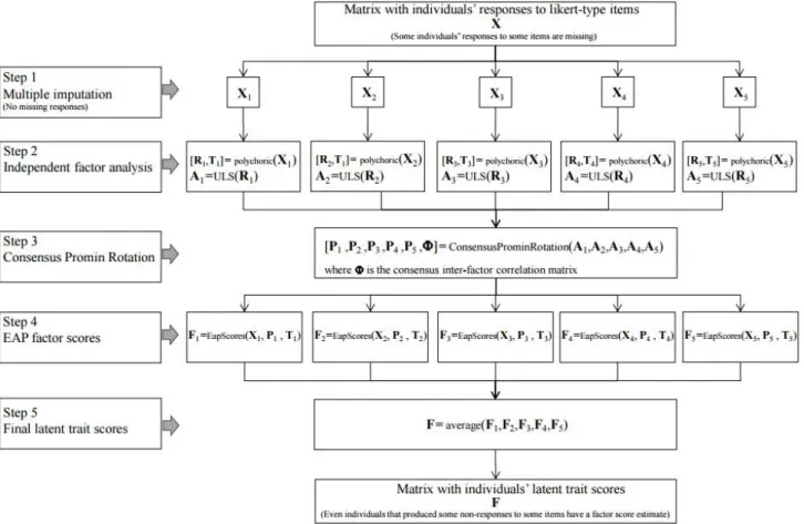
The procedure that we propose is based on five main steps that are explained in detail below and summarized in Figure
1. None of the analyses included in the five steps is new and they can be found in the literature. The merit of our pro-posal is to point out how they can be used to compute mul-tidimensional exploratory factor analysis when some re-sponses are missing.
Figure 1. Procedure to obtain estimates of latent trait scores for ordinal data when data is missing from the dataset.
Step 1: Multiple imputation
The problem that needs to be solved is how to fill in the missing values of a participant in a multidimensional psycho-logical test (i.e., scales that consist of a number of subscales) in which each subscale is made up of a number of Likert-type items. For this purpose, various MI approaches can be used. In our simulation studies presented below, we use two approaches: Hot-deck Multiple Imputation (HD-MI), and Predictive mean matching (PMM-MI).
Single hot-deck imputation was developed for item non-response in the Income Supplement of the Current Popula-tion Survey, initiated in 1947 (Ono & Miller, 1969). A recent review of different techniques of hot-deck imputation can be found in Andridge and Little (2010). Hot-deck replaces miss-ing values in incomplete cases (donees) with observed values from donors in the same data set to create a complete data set. In some versions, the donor is selected randomly from a
items is large (a typical situation in multidimensional scales); (b) a large sample is available from which potential donors can be taken; and (c) all the imputations will be in the range of specific values used in the Likert-type items.
Single hot-deck imputation can be generalized to become a multiple imputation procedure: Hot-deck Multiple Imputa-tion (HD-MI), also known as K-nearest-neighbors hot-deck imputation. This is an imputation technique in which missing values in incomplete cases (donees) are replaced with
ob-served values from donors in the same data set to create K
complete data sets. HD-MI has been shown to improve the simplest approaches, and it has remained a popular option in many applications (Aittokallio, 2010). Like single HD impu-tation, HD-MI is a simple and convenient procedure for dealing with missing responses.
Predictive mean matching (PMM) (Rubin, 1986) could at some extend be defined as a hot-deck imputation method:
the main difference is that observed values for Y are
re-gressed on a set of observed variables X. Then, predicted
values for Y are calculated for all Y using the regression
pa-rameters calculated for the observed data. Finally, missing Y
values are imputed using observed values of Y whose
pre-dicted values most closely match the prepre-dicted values of the respondents with missing data. The set of predictor variables
X to be used to predict variable Y must be correlated with
variable Y. Each variable Y to be imputed can use a different
set of predictor variables X.
When we applied HD-MI, we selected the K nearest
neighbors (i.e., the donors) to the donee. The selection was made taking into consideration all the individuals of the sample that produced responses for the same set of items as
the donee: the K participants with the lowest Euclidean
dis-tance are taken as the donors. Once the K donors for each
donee have been selected, K copies of the original data are
generated in which donees’ missing responses are replaced with the corresponding donors’ responses. PMM-MI uses
the procedure explained above to create K copies of data as
well. In this way, K complete versions of the data set are
ob-tained. In our simulation study presented below, we used K
= 5 with acceptable results.
As our approach is not related to a particular MI method, researchers can use the MI procedures that we tested in our simulation studies or others that are available in the litera-ture. MI can be computed by software packages such as
SPSS, R (see Amelia II package available at
http://gking.harvard.edu/amelia), or Matlab (for example,
function knnimpute available in Bioinformatics Toolbox).
Step 2: Independent exploratory factor analysis
Once the data have been multiply imputed, each copy is independently analyzed using EFA. As already explained, the nonlinear UVA is appropriate for analyzing the data. In the most usual approach (see e.g. Mislevy, 1986), the item thresholds are estimated from the marginals in the table and the tetrachoric/polychoric correlations are estimated from the joint frequency cells. So, routine factor analysis of the tetrachoric/polychoric correlation matrix provides the esti-mates of the loading values. In this way, for each copy of da-ta, we obtain (a) the item thresholds, (b) the polychoric cor-relation matrix, and (c) the matrix of loading values. It must
be noted that the decision on how many r factors to extract
(one factor for each latent trait) has to be the same for the K
copies of data. The factors can be extracted using Un-weighted Least Squares (ULS), for example. After this step,
K unrotated loading matrices Ak are obtained.
Researchers can use the R package polycor to compute
polychoric correlation matrices
(http://cran.r-project.org/web/packages/polycor/). In addition, the R package psych makes it possible to compute different factor loading estimates
(http://cran.r-project.org/web/packages/psych/).
Step 3: Consensus factor rotation
In EFA of a single dataset, the loading matrix is typically rotated to maximize factor simplicity (Kasier, 1974) using an orthogonal or an oblique rotation method. However, in this
step of the analysis, K loading matrices Ak need to be rotated.
In our situation, the independent rotation that maximizes
simplicity in each loading matrix Ak has an important
draw-back: the freedom of the final position of rotated factors means that the rotated factor solutions may turn out to be
non-comparable between the K copies of data. A (semi)
con-firmatory factor analysis would not have this drawback: the hypothetical loading matrix that is proposed in the
popula-tion model is used as a kind of target to the K factor
solu-tions. However, in an EFA such a common hypothesis (or target) does not exist. To avoid the drawback, the K factor
loading matrices Ak have to be simultaneously orthogonally
(or obliquely) rotated so that they are both (a) factorially simple, and (b) as similar to one another as possible. For the orthogonal rotation, Consensus Varimax can be computed (see, for example, Kiers, 1997). For the oblique rotation, Consensus Promin (Lorenzo-Seva, Kiers, & ten Berge, 2002) is available. Both consensus rotations are based on a
previ-ous Generalized Procrustes Rotation (GPR). Let Ak be the
set (k = 1…K) of unrotated loading matrices of order mr
obtained by factor analysis with m variables and r factors
re-tained. This set of loading matrices is orthogonally rotated by GPR (ten Berge, 1977) by minimizing,
Kk K
l
l l k k p
g
1 1
2 1
,...,
)
over S1,…, SK, subject to SkSk’ = Sk’Sk = I. So the set of
loading matrices AkSk shows optimal agreement in the least
squares sense. The Consensus Promin rotation consists of applying Promin (Lorenzo-Seva, 1999) to the mean of the
matched loading matrices AkSk, thus minimizing
with U subject to
diag
(
U
1U
1'
)
I
. The obliqueload-ing matrices Pk of order mr are computed as,
U
S
A
P
k
k k. (3)
As far as we know, neither Consensus Varimax nor Con-sensus Promin rotations have been specifically programmed
in R language. However, researchers can use the various R
packages available to obtain a consensus rotation. For
exam-ple, GPR is available in the procGPA package
(http://www.inside-r.org/packages/cran/shapes/docs/procGPA ), and Promin
rotation is available in the PCovR package
(http://www.inside-.org/packages/cran/PCovR/docs/pro-min; Vervloet et al., 2015). After the consensus rotation, pat-tern matrices of the K copies of data are comparable, and can be used to compute estimates of latent trait scores.
Step 4: Estimates of latent trait scores
Because the items in the psychological test are frequently Likert-type items, an appropriate procedure should be used
to estimate the r latent trait scores. One popular approach is
to compute expected a posteriori (EAP) estimators (Muraki & Engelhard, 1985). In the context of our multiple
imputa-tion method, EAP estimates of the r latent trait scores must
be computed for the K copies of the data. For each copy of
the data, the corresponding item scores (with donees’ miss-ing responses replaced with the correspondmiss-ing donors’ re-sponses), item thresholds, and the rotated loading matrix are
used to compute the r EAP scores. For each individual, K
EAP estimates are computed related to the r latent traits.
Although EAP factor scores are not frequently used in
applied research, they can be computed using an R package:
Latent Trait Models under IRT (ltm)
(http://www.inside-r.org/packages/cran/ltm/docs/factor.scores).
Step 5: Final latent trait scores
Once the K estimates of the r latent trait scores are
avail-able for each individual, the average of the K estimates of each individual is computed so that the final estimates of the
r latent trait scores can be obtained.
Simulation study based on a real dataset
In this section, we present an illustrative example of how the multiple imputation method followed by simultaneous rota-tion performs with a dataset in which missing data are artifi-cially introduced. The aim is to assess whether the imputa-tion method can obtain reasonably good estimators of the la-tent trait scores for incomplete data. The study has four main steps: (a) first, for a particular psychological test, it de-tects the pattern of missing values obtained in a real situa-tion; (b) second, it introduces missing data into a dataset that was initially complete; (c) then, it computes the estimates of the latent trait scores using the original dataset (i.e., the da-taset that is free of missing data), and the estimates of the la-tent trait scores after introducing artificial missingness; (d) and, finally, it compares the estimators obtained in both situ-ations to assess the performance of the imputation method proposed. In addition to the multiple imputation method, we included a simplistic alternative imputation method that is frequently used in real research. In the section below we de-scribe the simulation study in detail.
Obtaining missing-data patterns from incomplete data
To study the pattern of missing values in a real situation, a sample of 747 individuals (51% women) were administered the Overall Personality Assessment Scale (OPERAS) (Vigil-Colet et al., 2013). OPERAS is a short measure for the five-factor model personality traits: Extraversion (EX), Emotion-al Stability (ES), Conscientiousness (CO), Agreeableness (AG), and Openness to Experience (OE). Each personality trait is measured with 7 items, and the participant must indi-cate the level of agreement with a sentence by using a five-point scale that goes from “fully disagree” (1) to “fully agree” (5). The test was administered in the traditional paper-and-pencil format. A sentence at the end of the test remind-ed the participants to review the test so that they would spot missing data. Two participants had more than 10 missing values: as they left more than 25% of items unanswered, these two participants were eliminated from the sample.
Even though the respondents were reminded to review their responses, on 65 occasions (out of 26,145) an item was not answered. All scales had missing data (with frequencies ranging from 10 to 17), and the maximum number of miss-ing values was observed in EX. A total number of 55 indi-viduals had incomplete response patterns (7.4% of the sam-ple): 2 participants had 3 missing values, 6 participants had 2 missing values, and 47 participants had only 1 missing value. These outcomes were taken as the pattern of missing data to be observed in OPERAS in a real situation. This pattern is used in the next step to introduce artificial missing data into a complete data set.
OPERAS was administered to a second sample of 745 participants (34% women). However, this second sample an-swered an on-line format of the test. In this version of the test a single item was presented on a computer screen at a time, and the computer refused to continue with the next item until a response had been given. With the on-line ver-sion, it was impossible to skip questions (i.e., non-responses could not be produced by the responder). Please note that OPERAS was actually developed by its authors in both pa-per-and-pencil and on-line formats.
The aim was to artificially introduce missing data into this second sample using the missing-data patterns from the first sample. Specifically, we aimed to introduce the missing values in the same kind of participants as the set of partici-pants who had given non-responses in the first sample, and in exactly the same items. The first step was to select the 55 participants in the second sample that were most similar to the 55 participants with missing data in the first: we comput-ed the Euclidean distance of the responses of the first partic-ipant who produced non-response in the first sample with respect to the responses of the 745 participants in the second sample, and selected the participant in the second sample who was most similar to that participant in the first sample. Please note that the Euclidean distance was computed using only the items to which the participant in the first sample ac-tually produced a response. The second step was to artificial-ly introduce in the participant selected from the second sam-ple the same non-responses as the participant from the first sample (i.e., we deleted the responses in exactly the same items in which a non-response was observed). The proce-dure was replicated then for the second participant who pro-duced a non-response in the first sample, in order to select the most similar participant from the second sample (now of 744 participants), and the non-responses observed in the par-ticipant of the first sample were also introduced in the partic-ipant of the second sample. This two-step procedure was replicated until we had 55 participants in the second sample with exactly the same non-responses as the 55 participants in the first sample.
At this point we had (1) a sample of 745 participants that had not produced any non-responses, and (2) the same sam-ple in which it was suspected that 55 participants would have produced a non-response if the computer had allowed them to and who had had 65 non-responses artificially introduced (following the pattern of non-responses observed in the sample that was administered the paper-and-pencil format test). In the rest of the document, we shall refer to the first sample as the Full Response (FR) sample, and the second as the Artificial Non-Response (ANR) sample.
Computing the estimates of latent trait scores in the FR sample is a typical analysis that presents no difficulties. How-ever, computing estimates of latent trait scores in the ANR sample is impossible, unless a specific method is used to deal with non-responses. In the section below we compute EAP estimates in the FR sample and use multiple imputation to compute EAP estimates in the ANR sample. We also use a popular single imputation procedure to assess whether our multiple imputation improves the performance of this single imputation method.
Computing the estimates of the latent trait scores
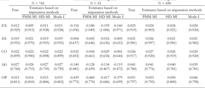
In order to compute the estimates of the latent trait scores in the FR sample, we used the program FACTOR (Lorenzo-Seva & Ferrando, 2013). We computed the poly-choric correlation matrix. The value of the KMO index was .87, which indicated that the correlation matrix was suitable for factor analysis. Optimal parallel analysis (Timmerman & Lorenzo-Seva, 2011) suggested that five factors could be ex-tracted. We extracted the five factors using unweighted least squares extraction, and obtained a CFI index of .98. To max-imize factor simplicity, we computed Promin rotation (Lo-renzo-Seva, 1999). The salient loading values of items in the rotated pattern were in accordance with the scales EX, ES, CO, AG, and OE. Finally, we computed the estimates of the five latent trait scores using the EAP estimator. The means and variances of the estimates are shown in Table 1, in the
columns labeled True. The table shows the statistics for the
Table 1. Mean and variances (printed in parentheses) for the true and the estimate of factor scores in the five personality factors.
Factor
Factor scores for the whole sample
N = 745
Factor scores for the subsample of individuals with missing data
N = 55
Factor scores for the subsample of individuals with-out missing data
N = 690
True imputation methods Estimates based on True imputation methods Estimates based on True Estimates based on imputation methods PMM-MI HD-MI Mode-I PMM-MI HD-MI Mode-I PMM-MI HD-MI Mode-I
EX 0.012 0.009 0.011 0.011 -0.154 -0.180 -0.159 -0.160 0.025 0.024 0.024 0.024 (0.929) (0.915) (0.928) (0.928) (1.036) (1.049) (1.006) (0.971) (0.919) (0.903) (0.921) (0.924)
ES 0.019 0.021 0.019 0.019 -0.004 -0.043 -0.016 -0.005 0.021 0.026 0.021 0.021 (0.955) (0.970) (0.955) (0.955) (0.637) (0.646) (0.636) (0.633) (0.981) (0.997) (0.981) (0.982)
CO 0.022 0.022 0.022 0.022 -0.032 -0.044 -0.029 -0.001 0.026 0.027 0.026 0.024 (0.899) (0.900) (0.898) (0.899) (0.692) (0.661) (0.654) (0.644) (0.917) (0.920) (0.919) (0.920)
AG 0.027 0.028 0.027 0.027 -0.140 -0.128 -0.134 -0.119 0.041 0.041 0.040 0.039 (0.760) (0.753) (0.759) (0.759) (0.481) (0.439) (0.467) (0.472) (0.780) (0.776) (0.781) (0.781)
OP 0.015 0.016 0.015 0.015 -0.439 -0.460 -0.417 -0.379 0.051 0.053 0.050 0.046 (0.811) (0.810) (0.806) (0.802) (0.775) (0.770) (0.686) (0.699) (0.797) (0.795) (0.800) (0.798)
In order to compute the estimates of the latent trait scores in the NR sample, we used three imputation methods to handle the missing data. The methods we used were:
1. Hot-Deck Multiple Imputation (HD-MI) (see above). We
used five copies of data. When subjecting the copies of the data to factor analysis, we used the same methods as the ones used when the FR sample was analysed. The on-ly difference was that instead of Promin rotation (useful when a single dataset is analyzed), we computed Consen-sus Promin rotation (useful when simultaneously rotating a number of datasets).
2. Predictive Mean Matching Multiple Imputation
(PMM-MI) (see above). Again, we used five copies of the data, and we used the same procedure as with HD-MI to
fac-tor analyze the K copies of data obtained.
3. Single imputation of the mode of the item (Mode-I). Any
missing value in the dataset was replaced with the mode of the item where the non-response was observed. We used the mode (instead of the mean or the median) be-cause we aimed to supply one of the answers that was al-ready on the response scale of the item (i.e., the values 1, 2, 3, 4, and 5). After the imputation of modes, we repli-cated the methods used when the FR sample was subject to factor analysis.
The means and variances of the estimates are shown in
Table 1, in the columns labeled PMM-MI, HD-MI and
Mode-I. As factor score estimates are computed from the
infor-mation obtained after the rotation of the factor loading ma-trix, a possible criticism of imputation is that it affects the es-timates related to the whole sample (not only the subsample of participants in which non-responses are observed), and consequently it might change the estimates of participants who do not have missing responses. To determine whether
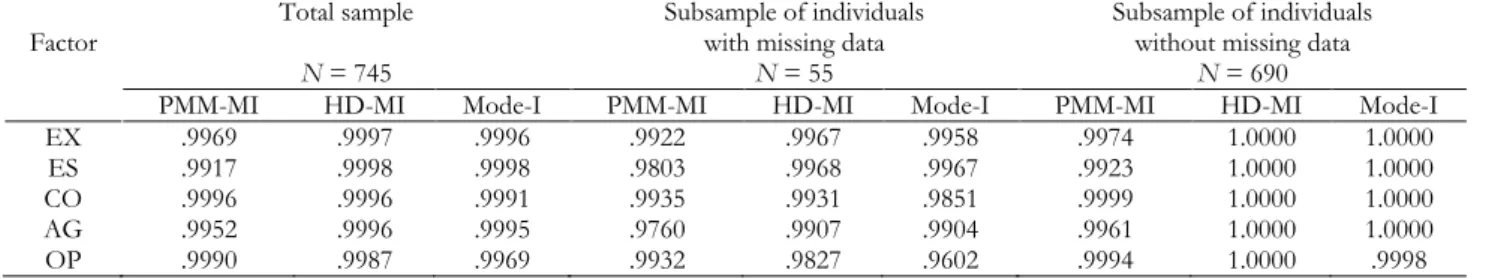
this criticism can be applied to our data analysis, Table 1 shows the statistics for (1) the whole sample, (2) the subsam-ple of individuals who have artificial missing data, and (3) the subsample of individuals who do not have missing data. As can be observed in the table, the three imputation methods closely replicated the same values (in terms of mean and var-iance) when analyzing the FR sample (i.e., when there are no missing data at all) in (a) the whole sample, and (b) the sub-sample of individuals who did not have missing data. How-ever, the estimates for the subsample of participants who had artificial missing data were generally replicated best when a multiple imputation method was used. As can be ex-pected, the worst imputation approach was Mode-I, whereas HD-MI and PMM-MI performed quite similarly. Table 2 shows the correlations between (a) the factor score estimates obtained in the FR sample (i.e., when there were no missing data), and (b) the factor score estimates obtained in the NR sample (i.e., when artificial missing data were introduced into the dataset). In terms of correlation, HD-MI performed slightly better than the others.
zero), whereas the more homogenous bias was observed for PMM-MI (in terms of variance and RMSR). When the sub-sample of participants without missing data was considered, the three imputation methods produced very accurate
esti-mates. However, PMM-IM was the approach that showed the largest RMSR: in this regard, PMM-IM seems to be the method that most affected the factor score estimates of the participants without missing data.
Table 2. Correlations between the true scores and the estimates based on different imputation methods.
Factor Total sample N = 745
Subsample of individuals with missing data
N = 55
Subsample of individuals without missing data
N = 690
PMM-MI HD-MI Mode-I PMM-MI HD-MI Mode-I PMM-MI HD-MI Mode-I EX .9969 .9997 .9996 .9922 .9967 .9958 .9974 1.0000 1.0000 ES .9917 .9998 .9998 .9803 .9968 .9967 .9923 1.0000 1.0000 CO .9996 .9996 .9991 .9935 .9931 .9851 .9999 1.0000 1.0000 AG .9952 .9996 .9995 .9760 .9907 .9904 .9961 1.0000 1.0000 OP .9990 .9987 .9969 .9932 .9827 .9602 .9994 1.0000 .9998
Table 3. Descriptive statistics of estimation bias (estimate score minus true score) for different imputation methods.
Statistics with incomplete response patterns Subsample of individuals with complete response patterns Subsample of individuals
N = 55 N = 690
PMM-MI HD-MI Mode-I PMM-MI HD-MI Mode-I
Mean -0.056 0.024 0.111 0.0012 -0.0006 -0.0006 95% CI (-0.104 ; -0.007) (-0.028 ; 0.077) (0.043 ; 0.180) (-0.001 ; 0.004) (-0.001 ; 0.000) (-0.001 ; 0.000) Variance 0.037 0.043 0.074 0.0057 0.0002 0.0002
RMSR 0.200 0.208 0.292 0.076 0.013 0.016
Simulation study based on artificial datasets
On the basis of the theoretical considerations and results from research discussed in the sections above, we hypothe-size that our multiple imputation approach will outperform the single imputation approach when used to estimate true factor scores. To study the comparative performance of two multiple imputation procedures (HD-MI and PMM-MI) and estimate the true factor score of individuals under different circumstances, we performed a simulation study based on ar-tificial data.
Data construction
The simulated data were generated with a linear common factor model, where the resulting continuous variables were categorized to yield ordered polytomous observed variables. The linear common factor model included both major and minor factors, as may well be the case with real-world data, on the basis of the middle model by Tucker, Koopman and Linn (1969). This approach was adopted in earlier research on the common factor model (see for example, Timmerman & Lorenzo-Seva, 2011). In the simulation study, the
popula-tion correlapopula-tion matrix of the continuous variables R*pop was
taken as
R*pop = wmamamama´ + wmimimi´ + wun IJ, (4)
where ma (J Qma) and mi (J Qmi) are major and minor
loading matrices, respectively, with Qma and Qmi being the
number of major and minor factors, and J the number of
ob-served variables; ma (Qma Qma) is the inter-factor
correla-tion between major factors; IJ (J J) is the identity matrix,
reflecting the covariance matrix of the unique parts of the variables; wma, wmi and wun are weights that make it possible to
manipulate
ma2 ,
mi2 and
un2 , the variances of thema-jor, minor and unique parts of the correlation matrix, respec-tively. In our study, these variances were kept constant so
that
ma2 =.64, and
mi2 =.10. In addition, the number ofmajor and minor factors was also kept constant: we consid-ered two major factors and six minor factors. The inter-factor correlation between major inter-factors was systematically
.30. Each simulated continuous data matrix X* (NJ), with
sample size N, was obtained by randomly drawing N vectors
from a multivariate normal distribution N(0, R*pop).
Subse-quently, each element xnj of the polytomous simulated data
matrix X (NJ) was obtained from the element
x
*nj of thecontinuous data matrix X* using prespecified thresholds τc(τc
= τ0,…,τC, with C= 5 the number of response categories),
with xnj = c if τc1xnj* τc. In real situations the item
re-sponses are non-symmetrically distributed so the distribution of the variables was manipulated to be systematically skewed in our datasets. For each single factor, half of the variables were skewed in the opposite direction to mimic differences in item difficulty in real scales and the thresholds were cho-sen such that the expected proportion of observations in
cat-egories c=1,…,C were [0.05, 0.60, 0.20, 0.10, 0.05].
empirical research. The sample size was varied (N = 500, 1,000 and 2,000) and the number of observed variables per major factor was also varied (M = 5 and 10). This means that, as the number of major factors was kept constant to 2,
the number of observed variables in the model was J=10 and
20.
For each X, we computed the estimated latent trait
scores as follows: (a) we computed the corresponding poly-choric correlation matrix R; (b) we extracted two factors us-ing unweighted least squares factor analysis, and (c) we com-puted estimated latent trait scores using the EAP estimator
for each individual in X. These estimated latent trait scores
were considered the true estimated latent trait scores (t) that
would be obtained if the data contained no missing values.
Simulation of artificial missing data
Once data matrix X was available, we introduced different
amounts of artificial missing data in order to obtain Y (i.e.,
the same dataset as X, but with missing data). The
propor-tion of missing data was manipulated to be G=.05, .10, and
.15. The three mechanisms that underlie the missing data process (MCAR, MNAR, and MAR) were simulated in order to produce data with artificial missing data. To generate
MCAR data, for each xij value in X, a uniform number
be-tween 0 and 1 (U) was randomly drawn. If the value of U was less than or equal to G, the item response yij was deleted.
To generate MNAR data, we computed the total scale score (S) of each individual as the addition of the observed
re-sponses of each participant in X. Then we computed
P(missing|S)=G(1-(S)), where (S) is the additive inverse of the normal cumulative density function. Once
P(missing|S) had been calculated, a uniform number
be-tween 0 and 1 (U) was randomly drawn. If the value of U
was less than or equal to P(missing|S), the item response yij
was deleted. To generate MAR data, we computed a
normal-ly distributed variable V that was correlated .5 with t. Then
we computed P(missing|V)=G(1-(V)), where (V) is the additive inverse of the normal cumulative density function.
Once P(missing|V) had been calculated, a uniform number
between 0 and 1 (U) was randomly drawn. If the value of U
was less than or equal to P(missing|V), the item response yij
was deleted.
It must be noted that from each matrix X (i.e., a matrix of individuals’ responses without missing data), 9 different matrices Y (i.e., a matrix of individuals’ responses with
miss-ing data) were computed: 3 different values of G 3
miss-ing data mechanisms.
Imputation of missing data
Once matrices Y were available, we proceeded to apply the
same imputation methods that we had used in the previous simulation study: Hot-Deck Multiple Imputation (HD-MI), Predictive Mean Matching Multiple Imputation (PMM-MI), and Single imputation of the mode of the item (Mode-I). For each Y, we computed the estimated latent trait scores as fol-lows: (a) we computed the corresponding polychoric correla-tion matrix; (b) we extracted two factors using unweighted least squares factor analysis, and (c) we computed estimated latent trait scores using the EAP estimator for each individu-al in each Y. These estimated latent trait scores were consid-ered the estimated latent trait scores () that could be ob-tained when the data contain missing values.
Dependent variable
We computed 500 replicates of the study. This resulted in 2
(number of observed variables per major factor) 3
(per-centage of missing responses) 3 (mechanism to produce
missing responses) 500 (replicates) = 27,000 simulated data
sets with artificially introduced missing responses. As the size
of the datasets with missing responses was N=500, 1000, or
2,000, the number of participants simulated in the study was 31,500,000. For each participant, the estimated latent trait scores were computed for both factors in each data set (i.e., a total of 64,000,000 estimated latent trait scores were com-puted), where the missing values were imputed using the three approaches discussed above: HD-MI, PMM-MI and Mode-I. To assess the performance of each imputation ap-proach, we computed the bias of the estimated latent trait scores: true estimated latent trait scores minus estimated
la-tent trait scores (t − ). To assess the accuracy, we
comput-ed the average bias. To assess the efficiency, we computcomput-ed the standard deviation of bias.
Results and conclusion of the simulation
study
Table 4. Average of bias obtained in the simulation study based on artificial data. Standard deviations of bias are printed in parenthesis.
Condition Mode-I HD-MI PMM-MI
Overall 0 .003037 (.1825) 0 .000126 (.1477) 0 .000580 (.1548)
Missing-response mechanism MCAR 0 .001922 (.1764) 0 .000121 (.1422) 0 .000429 (.1492) MAR 0 .004584 (.1904) 0 .000376 (.1565) 0 .000583 (.1626) MNAR 0 .002604 (.1805) 0 .000120 (.1439) 0 .000728 (.1522)
Sample Size 500 0 .002724 (.1820) 0 .000194 (.1507) 0 .000493 (.1547) 1000 0 .003102 (.1827) 0 .000040 (.1474) 0 .000635 (.1539) 2000 0 .003082 (.1826) 0 .000152 (.1470) 0 .000574 (.1552)
Number of items per factor (m/r) 5 0 .001710 (.1963) 0 .000051 (.1562) 0 .000670 (.1697) 10 0 .004364 (.1677) 0 .000302 (.1386) 0 .000491 (.1382)
Percentage of missing responses 5 0 .001827 (.1248) 0 .000122 (.0960) 0 .000521 (.1031) 10 0 .003195 (.1811) 0 .000044 (.1440) 0 .000705 (.1512) 15 0 .004089 (.2271) 0 .000543 (.1884) 0 .000514 (.1959)
The most difficult situations for HD-MI were when (a) the missing data mechanism was MAR, (b) the number of observed variables per factor was large, and (c) the percent-age of missing data was large. PMM-MI showed a consistent tendency to overestimate the true values. The most difficult situations of PMM-MI were when (a) the missing data mech-anism was MNAR, (b) the number of observed variables per factor was low, and (c) the percentage of missing responses was large.
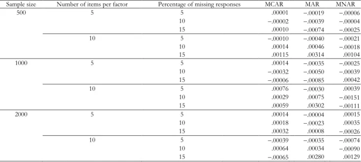
Overall, these results show that single imputation of missing values should not be used (i.e., Mode-I in our simu-lation study), and that multiple imputation based on the Hot-Deck approach (i.e., HD-MI in our simulation study) was the most accurate and efficient approach. In order to get further insight into the interaction among the conditions used in the
simulation study, we further studied the results obtained with the most successful approach (i.e., HD-MI). Table 5 shows the average bias in the various conditions related to HD-MI. When missing responses were due to MAR, the bias was largest when the number of variables per factor was large and the percentage of missing responses was large; this bias was even greater when the sample size was low. When miss-ing responses were due to MCAR, the bias was largest when the sample size was low, the number of items per factor large, and the percentage of missing responses large. When missing responses were due to MNAR, the bias was lower than when missing responses were due to MAR or MCAR. However, bias increased when the percentage of missing re-sponses was large, the number of items per factor was large, and the sample size was large.
Table 5. Average of bias obtained related to HD-MI approach depicted for manipulated conditions of the simulation study.
Sample size Number of items per factor Percentage of missing responses MCAR MAR MNAR
500 5 5 .00001 .00019 .00006
10 .00002 .00039 .00004
15 .00010 .00074 .00025
10 5 .00010 .00040 .00021
10 .00014 .00046 .00018
15 .00115 .00314 .00104
1000 5 5 .00014 .00035 .00025
10 .00032 .00050 .00039
15 .00006 .00085 .00042
10 5 .00076 .00030 .00039
10 .00029 .00075 .00151
15 .00059 .00302 .00111
2000 5 5 .00014 .00004 .00015
10 .00018 .00023 .00035
15 .00032 .00008 .00026
10 5 .00039 .00035 .00074
10 .00064 .00034 .00090
Discussion
In EFA, researchers usually have to deal with missing data: for some reason, some participants leave some items unan-swered. While the performance of multiple imputation with continuous data has been extensively studied, much less work has been done on the performance of multiple imputa-tion with ordinal data (Finch, 2008). We suggest how the multiple imputation approach can be used in the context of EFA. It should be pointed out that while multiple imputation has been studied in unidimensional situations (see, for exam-ple, Finch, 2008, 2011), our approach is useful in multidi-mensional situations: to our knowledge no previous work has been done on this specific situation, which is frequent in real applied research. The key step in our procedure is to
simul-taneously rotate the K copies of data obtained after multiple
imputation, so that the K factor scores for each individual are
comparable (i.e., the average between the K factor score
es-timates of an individual can be computed to obtain the final factor score estimation of the individual).
We carried out simulations based on real data and artifi-cial datasets. In the study with real data, we used two sam-ples: one sample in which a personality test was administered in the traditional pencil and paper format, and which had missing data; and a sample in which the same personality test was administered with computer software that did not allow for non-responses. The results in this simulation study sug-gested that our approach was actually successful, and pro-duced better factor score estimates than single imputation methods.
In the study with the artificial dataset, we manipulated three missing data mechanisms (MCAR, MAR, and MNAR), the sample size, the proportion of items per factor, and the percentage of missing responses. The results of this study suggest that single imputation (Mode-I in our study) is not an advisable option, and that HD-MI is the most accurate and efficient of the approaches used. HD-MI was less accurate when MAR was the mechanism responsible of the nonre-sponses, than when MCAR or MNAR were the responsible mechanisms of the nonresponses. In the same way, PMM-MI was less efficient when MAR was the mechanism respon-sible of the nonresponses. The conclusion is that, of the three missing data mechanisms, MAR seems to be the most difficult one to deal with.
In the simulation study, our approach was tested with two multiple imputation methods: Hot-deck (Ono & Miller, 1969), and Predictive Mean Matching (Rubin, 1986). Overall, Hot-deck Multiple Imputation seemed to perform slightly better in our dataset than Predictive Mean Matching Multiple Imputation. In addition, it should be pointed out that single imputation of the mode the items was the approach that per-formed worst.
Our paper proposes a multiple imputation approach to deal with missing responses, with particular focus on the procedure for obtaining latent trait estimates. However, oth-er approaches can be found in the litoth-erature. Yuan, Marshall
and Bentler (2002) proposed a unified approach to explora-tory factor analysis that included missing values and was based on generalizing the maximum likelihood approach un-der constraints in orun-der to assess statistical properties of es-timates of factor loadings and error variances. However, they did not specifically deal with the difficulty of computing fac-tor scores. Yuan and Lu (2008) provided the theory and ap-plication of the 2-stage maximum likelihood procedure for structural equation modeling with missing data (see also Yu-an & ZhYu-ang, 2012, Yu-and YuYu-an & Savalei, 2014). Their ap-proach is especially advisable if the data mechanism is MAR. If the missing data mechanism is unknown, they advise that auxiliary variables be included in the analysis to make the missing data mechanisms more likely to be MAR. From our point of view, it cannot be easily assumed that the MAR mechanism plays a role in nonresponses to psychological tests. A psychological test is composed of a number of items: even if all the items in the same scale are expected to have a latent variable in common, each item is related to a specific facet of the latent variable. What is more, if two items are re-lated to exactly the same facet of a latent variable, then one of the items is redundant and should not have been in the test from the very beginning. The response to a psychologi-cal item may be missing because of the content of the specif-ic facet the item is measuring or some specifspecif-ic characteristspecif-ic of the item itself (for example, the item includes a word that is ambiguous for some individuals). None of these character-istics depends on the other items in the scale. From this point of view, the factor model cannot be estimated only from the available data. For this reason, the MAR nism cannot easily be assumed as the nonresponse mecha-nism in the context of psychological tests. Our proposal does not assume any missing data mechanism: it is based on shar-ing the information given by the participants who responded to the item for which a response was missing. The only as-sumption in our approach is that individuals who had already produced similar responses would tend to produce responses that were similar to those of the unanswered items. This as-sumption is more acceptable in the context of psychological tests.
Wolkowitz and Skorupski (2013) proposed a method for imputing response options for missing data based on multi-ple-choice assessments but state that it is intended for test development planning purposes, and that additional research is needed before it can be used to operationally score a test.
There are several R language packages available to re-searchers interested in computing our approach to missing values in the context of multidimensional EFA. We have
programmed our approach in Matlab: we shall be glad to
share our Matlab functions with interested researchers.
Final-ly, we have implemented the multiple imputation methods studied in this paper in FACTOR 10.1 (Lorenzo-Seva & Fer-rando, 2013), a stand-alone program for Windows for fitting exploratory and semiconfirmatory factor analysis and IRT
Models. The program, a demonstration, and a short manual are available at:
http://psico.fcep.urv.cat/utilitats/factor .
Acknowledgements.- The research was partially supported by a grant from the Catalan Ministry of Universities, Research and the Information Society (2014 SGR 73) and by a grant from the Span-ish Ministry of Education and Science (PSI2014-52884-P).
References
Aittokallio, T. (2010). Dealing with missing values in large-scale studies: mi-croarray data imputation and beyond. Briefings in bioinformatics, 11, 253-264. doi:10.1093/bib/bbp059.
Andridge, R. R., & Little, R. J. (2010). A review of Hot Deck imputation for survey non-response. International Statistical Review, 78, 40-64. doi:10.1111/j.1751-5823.2010.00103.x.
Ayala, R. J., Plake, B. S., & Impara, J. C. (2001). The impact of omitted re-sponses on the accuracy of ability estimation in item response theory.
Journal of educational measurement, 38, 213-234. doi:10.1111/j.1745-3984.2001.tb01124.x.
Bock, R. D., & Aitkin, M. (1981). Marginal maximum likelihood estimation of item parameters: an application of the EM algorithm. Psychometrika,
46, 443-459. doi:10.1007/BF02293801.
Chen, J., & Choi, J. (2009). A comparison of maximum likelihood and ex-pected a posteriori estimation for polychoric correlation using Monte Carlo simulation. Journal of Modern Applied Statistical Methods, 8(1), 32. Cuesta, M., Fonseca, E., Vallejo, G., & Muñiz, J. (2013). Datos perdidos y
propiedades psicométricas en los test de personalidad. Anales de Psi-cología, 29(1), 285-292. doi:10.6018/analesps.29.1.137901.
DeMars, C. (2003, April). Missing data and IRT item parameter estimation. Paper presented at the annual meeting of the American Educational Re-search Association, Chicago, IL.
Ferrando, P.J. & Lorenzo-Seva, U. (2013). Unrestricted item factor analysis and some relations with item response theory. Technical Report. Department of Psychol-ogy, Universitat Rovira i Virgili, Tarragona. Retrieved from http://psico.fcep.urv.cat/utilitats/factor.
Finch, H. (2008). Estimation of item response theory parameters in the presence of missing data. Journal of Educational Measurement, 45, 225-245. doi:10.1111/j.1745-3984.2008.00062.x.
Finch, H. (2011). The Use of Multiple Imputation for Missing Data in Uni-form DIF Analysis: Power and Type I Error Rates. Applied Measurement in Education, 24, 281-301. doi:10.1080/08957347.2011.607054. Graham, J. W. (2009). Missing data analysis: Making it work in the real
world. Annual review of psychology, 60, 549-576. doi: 10.1146/annurev.psych.58.110405.085530
Huisman, M., & Molenaar, I. W. (2001). Imputation of missing scale data with item response models. In Essays on item response theory (pp. 221-244). Springer New York. doi:10.1007/978-1-4613-0169-1_13. Johnson, D. R., & Young, R. (2011). Toward best practices in analyzing
da-tasets with missing data: Comparisons and recommendations. Journal of Marriage and Family, 73, 926-945. doi:10.1111/j.1741-3737.2011.00861.x. Kaiser, H. F. (1974). An index of factorial simplicity. Psychometrika, 39,
31-36. doi:10.1007/BF02291575
Kiers, H. A. (1997). Techniques for rotating two or more loading matrices to optimal agreement and simple structure: A comparison and some technical details. Psychometrika, 62, 545-568. doi:10.1007/bf02294642. Kleinke, K., Stemmler, M., Reinecke, J., & Lösel, F. (2011). Efficient ways
to impute incomplete panel data. AStA Advances in Statistical Analysis,
95, 351-373. doi:10.1007/s10182-011-0179-9.
Lorenzo-Seva, U. (1999). Promin: a method for oblique factor rotation.
Multivariate Behavioral Research, 34, 347-365. doi:10.1207/S15327906MBR3403_3.
Lorenzo-Seva, U., & Ferrando, P. J. (2013). FACTOR 9.2: A Comprehen-sive Program for Fitting Exploratory and Semiconfirmatory Factor
Analysis and IRT Models. Applied Psychological Measurement, 37, 497-498. doi:10.1177/0146621613487794.
Lorenzo-Seva, U.; Kiers, H. A. L.; ten Berge, J. M. F. (2002). Techniques for oblique factor rotation of two or more loading matrices to a mix-ture of simple strucmix-ture and optimal agreement. British Journal of Mathe-matical & Statistical Psychology, 55, 337-360. doi:10.1348/000711002760554624.
Mislevy, R. J. (1986). Recent developments in the factor analysis of categor-ical variables. Journal of educational statistics, 11, 3-31. doi:10.3102/10769986011001003.
Moustaki, I., Joreskog, K., & Mavridis, D. (2004). Factor models for ordinal variables with covariate effects on the manifest and latent variables: a comparison of LISREL and IRT approaches. Structural equation model-ling, 11, 487-513. doi:10.1207/s15328007sem1104_1.
Muraki, E., & Engelhard, G. (1985). Full-information item factor analysis: Applications of EAP scores. Applied Psychological Measurement, 9, 417-430. doi:10.1177/014662168500900411.
Muthén, L. K., & Muthén, B. O. (1998-2011). Mplus User's Guide. (Sixth ed.). Los Angeles, CA: Muthén & Muthén.
Myers, T. A. (2011). Goodbye, listwise deletion: Presenting hot deck impu-tation as an easy and effective tool for handling missing data. Communi-cation Methods and Measures, 5(4), 297-310. doi:10.1080/19312458.2011.624490.
Ono, M., & Miller, H. P. (1969). Income nonresponses in the current popu-lation survey. In Proceedings of the Social Statistics Section, American Statisti-cal Association, 277-288.
Rässler, S., Rubin, D. B., & Zell, E. R. (2013). Imputation. Wiley Interdiscipli-nary Reviews: Computational Statistics, 5, 20-29. doi:10.1002/wics.1240. Rubin, D. B. (1976). Inference and missing data. Biometrika, 63, 581-592.
doi:10.1093/biomet/63.3.581.
Rubin, D. B. (1978). Multiple imputations in sample surveys-a phenomeno-logical Bayesian approach to nonresponse. In Proceedings of the Sec-tion on Survey Research Methods, American Statistical AssociaSec-tion, 20-34.
Rubin, D. B. (1986). Statistical matching using file concatenation with ad-justed weights and multiple imputations. Journal of Business & Economic Statistics, 4, 87-94. doi:10.1080/07350015.1986.10509497.
Schafer, J. L., & Graham, J. W. (2002). Missing data: our view of the state of the art. Psychological methods, 7, 147. doi:10.1037/1082-989x.7.2.147. Schlomer, G. L., Bauman, S., & Card, N. A. (2010). Best practices for
miss-ing data management in counselmiss-ing psychology. Journal of Counseling Psy-chology, 57, 1-10. doi:10.1037/a0018082.
Siddique, J., & Belin, T. R. (2007). Multiple imputation using an iterative hot-deck with distance-based donor selection. Statistics in medicine, 27, 83-102. doi:10.1002/sim.3001.
Sijtsma, K., & Van der Ark, L. A. (2003). Investigation and treatment of missing item scores in test and questionnaire data. Multivariate Behavioral Research, 38, 505-528. doi:10.1207/s15327906mbr3804_4.
Ten Berge, J. M. (1977). Orthogonal Procrustes rotation for two or more matrices. Psychometrika, 42, 267-276. doi:10.1007/BF02294053. Timmerman, M.E.; Lorenzo-Seva, U. (2011). Dimensionality assessment of
ordered polytomous items with parallel analysis. Psychological Methods,
Tucker, L. R., Koopman, R. F., & Linn, R. L. (1969). Evaluation of factor analytic research procedures by means of simulated correlation matri-ces. Psychometrika, 34, 421-459. doi:10.1007/BF02290601.
Vervloet, M., Kiers, H. A., Van den Noortgate, W., & Ceulemans, E. (2015). PCovR: An R Package for Principal Covariates Regression.
Journal of Statistical Software, 65, 1-14. doi:10.18637/jss.v065.i08. Vigil-Colet, A., Morales-Vives, F., Camps, E., Tous, J., & Lorenzo-Seva, U.
(2013). Development and validation of the Overall Personality Assess-ment Scale (OPERAS). Psicothema, 25, 100-106. doi:10.7334/psicothema2011.411.
Wolkowitz, A. A., & Skorupski, W. P. (2013). A Method for Imputing Re-sponse Options for Missing Data on Multiple-Choice Assessments.
Educational and Psychological Measurement, 73, 1036-1053. doi:10.1177/0013164413497016.
Yuan, K. H., & Lu, L. (2008). SEM with missing data and unknown popu-lation distributions using two-stage ML: Theory and its application.
Multivariate Behavioral Research, 43, 621-652. doi:10.1080/00273170802490699.
Yuan, K. H., & Savalei, V. (2014). Consistency, bias and efficiency of the normal-distribution-based MLE: The role of auxiliary variables. Journal of Multivariate Analysis, 124, 353-370. doi:10.1016/j.jmva.2013.11.006. Yuan, K. H., & Zhang, Z. (2012). Robust structural equation modeling with
missing data and auxiliary variables. Psychometrika, 77, 803-826. doi:10.1007/s11336-012-9282-4.
Yuan, K. H., Marshall, L. L., & Bentler, P. M. (2002). A unified approach to exploratory factor analysis with missing data, nonnormal data, and in the presence of outliers. Psychometrika, 67, 95-121. doi:10.1007/BF02294711.