Vol 7, No 7 (2017)

(1)

Research Article

July

2017

Computer Science and Software Engineering

ISSN: 2277-128X (Volume-7, Issue-7)

Case Study: Analysis and Predictions of Shipment Load in

Festive Season

Megha Chhabra*

Department of Computer Science and Engineering, Sharda University, Greater Noida, Uttar Pradesh, India

DOI: 10.23956/ijarcsse/SV7I5-0325

Abstract— A time-phased forecasting in rest of the year has a huge impact shipping costs, however during a festive season of the year, well predicted and analyzed re-engineering of shipment load plays a major role in bringing up sales. The major concern of the customer is to get delivery on-time, whereas that of the wholesaler / retailer is to provide delivery without any complaint in order to retain the customer. In the framework of competitive supply chain market, necessary accurate Shipping load forecasting tools are required. With the focus of improving prediction accuracy, this case study presents use of Time-series models, multiplicative decomposition model (MDM) and smoothening techniques, on shipping load demand of Arora-Ludhiana-Handlooms during festive seasons for short-term forecasting.

Keywords— Shipment load, forecasting, time series analysis, trend adjustment.

I. INTRODUCTION

Supply chain managements involve huge planning horizon for demand forecasting. For the purpose they use forecast systems for initial forecast followed by judgmental adjustment by the company experts to adjust exceptional events in the planning process. The manual adjustments made raise questions related to improvement of accuracy and type of adjustments made. Effective Short-term forecasting is important for improving supply chain management [24], [27], irrespective of the type of business.

Multiple applications of the prediction analysis and adjustment behavior in prediction accuracy can be seen in past few years [14]-[16], [18]-[20]. According to the literature of economic forecasting, accuracy of the statistical decisions can be improved when experts consider the changes in the statistical models according to the changes coming from occurrence of special events [1]-[8], [10], [11] and [22]-[23] showed that the suggested judgmental adjustments tend to improved accuracy marginally but may also introduce bias. Since it‘s a human added knowledge as a judgement factor, it is more likely to make error in level of adjustment and make room for error as experimental evidences suggest [11], [25]-[26] Forecasters make decisions on the basis of noisy and randomly fluctuating events in time series [9].

Several methods, techniques have been used in literature to forecast load demands. Two time-series models, multiplicative decomposition and the smoothing technique, are used profoundly in various business sectors. An exponentially weighted moving average is a means of smoothing random fluctuations that has the following desirable properties: (1) declining weight is put on older data, (2) it is extremely easy to compute, and (3) minimum data is required [18]. Exponential smoothing methods are widely used in industry. Their popularity is due to several practical considerations in short-range forecasting [21].

This study presents effect of seasonal demand on prediction methodology of above mentioned models using reference data of handlooms business sector for predicting shipment load for Arora-Ludhiana-Handlooms Company. The proposed methods are used to predict one month‘s demand. The outcome of both models is analyzed and accuracy is compared.

II. TIME SERIES MODELS

A time series is sequential nature of data produced during a certain period of time. Assuming no major disrupting to critical parameters of a recurring event, the future prediction is always related to past data. Two time-series analysis models, namely, multiplicative decomposition and the smoothing technique use the dependency of future data to the past events, and model the behavior as follows:

A. Multiplicative decomposition model (MDM)

Four components, trend component T(t), seasonal component S(t), cyclic component C(t) and random component R(t), MDM models time series as follows:

X(t)= T(t) * S(t) * C(t) * R(t)

C(t) is during periodic for a year or more, hence is not applicable in short-term forecasting. Therefore, X(t)= T(t) * S(t) * R(t)

B. Smoothing Techniques

(2)

ISSN(E): 2277-128X, ISSN(P): 2277-6451, DOI: 10.23956/ijarcsse/SV7I5-0325, pp. 491-495

 Moving averages: A moving average (MA) is an average of the data provided for certain number of time period.

The method is called ―moving‖ because it is obtained using summing and averaging the values from a given number of periods say n, each time deleting the oldest value and adding the new one.

Moving average ( MAt+1 ) = Dt-i/n (3)

Where t= current period

D= actual data exchanged each period. n = length of the time period.

 Weighted moving Average (WMA): In MA each observation is given equal weightage, which in real situations

is less likely to occur. It may be desired to place more weight on certain period of time than others. When certain inputs are weighted differently than others, the moving average outcome of those inputs is called weighted moving average (WMA). In this case, different values may be assigned to compute a weighted average of the most recent n values.

Hence, Weighted Moving average

(WMAt+1) =∑(Weight for period n) ( data value in period n)/∑Weights (4)

 Exponential smoothing Technique: A type of MA forecasting technique which weighs past data from previous

time periods with exponentially decreasing importance in the forecast so that the most recent data carries more weight in the moving average. For finding trend effect, adjusted exponential smoothing gives a better answer. Hence,

Trend adjusted forecast (Ft)adj = Ft + (1- β)/β * Tt (5)

And Ft = Ft-1 + α(Dt-1 - Ft-1)

Where (Ft)adj = trend-adjusted Forecast

Ft = Simple exponential smoothing factor

β = Smoothing constant for trend

Tt = exponentially smoothed trend factor

III. EXPERIMENTATION

In order to fit the seasonal component, extent of seasons is fixed for two weeks duration. For example, Arora-Ludhiana-Handlooms, Ludhiana manufacturers tend to see a huge impact on sale during Diwali, Baisakhi etc. This sections analyses the trend variation during a month in order to predict future shipment load. Data for 1 months prior to 5 festivals is chosen to accommodate major days of festivals range of the region. Each month‘s shipment load is recorded and analyzed to forecast next festive season‘s shipment load for the given market trend.

A. Data

The data is collected for the festive season‘s months of Punjab for Arora-Ludhiana-Handlooms business. Table 1 is organized structure of observed shipment load for the festive season of Lohri (Jan‘16), Holi (March‘16), Vaisakhi (April‘16), Rakhsha-Bandhan (August‘16), Krwachauth-(Sep-Oct‘16), Diwali (Oct-Nov‘16), E-id (Oct-Nov‘16), Guru-Nanak Jayanti (Nov‘16), Christmas (Dec-16). All three Smoothing averages are applied on the data collected and outcome is predicted for festive season of Lohri (Jan‘17).

Table 1. Observed shipment load for the festive season of 2016 for Arora-Ludhiana-Handlooms Business sector.

Festive season Month Observed Shipment Load (Average Units per pack of Handlooms Retailer )

Lohri (Jan‘16) 500

Holi (March‘16) 130

Vaisakhi (April‘16) 200

Rakhsha-Bandhan (August‘16) 250

Krwachauth (Sep-Oct‘16) 450

Diwali (Oct-Nov‘16) 300

E-id (Oct-Nov‘16) 450

Guru-Nanak Jayanti (Nov‘16) 100

Christmas (Dec-16) 500

Lohri (Jan‘17) 480

 Moving averages: Here the moving average (MA) is an average of the data provided for observed shipment

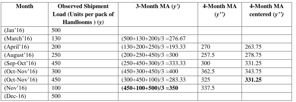
load of Arora-Ludhiana-Handlooms for months of Jan‘16 to Dec‘16. Table 2 shows 3-month and 4-month MA. The outcome MA3 and MA4 are the two averages predicting the shipment load for festive season of Lohri

(Jan‘17) using Moving averages. MA3= 350 and MA4 =331.25 for Jan‘17 i.e. Lohri season which is given to be

most impactful season. Table 1. Shows the observed value of Lohri as 480. This shows MA3 gives relatively

(3)

 Weighted moving Average (WMA): The owner of the sale-market decides to weigh the past three months sales

as follows:

Weights Months

3/6 Last Month

1/6 Two months ago

2/6 Three Months ago

Table 2: Calculation of Trend and short-term Fluctuations

Month Observed Shipment Load (Units per pack of

Handlooms ) (y)

3-Month MA (y’) 4-Month MA (y’’)

4-Month MA centered (y’’)

(Jan‘16) 500

(March‘16) 130 (500+130+200)/3 =276.67

(April‘16) 200 (130+200+250)/3 =193.33 270 263.75

(August‘16) 250 (200+250+450)/3 =300 257.5 278.75

(Sep-Oct‘16) 450 (250+450+300)/3 =333.33 300 331.25

(Oct-Nov‘16) 300 (450+300+450)/3 =400 362.5 343.75

(Oct-Nov‘16) 450 (300+450+100)/3 =283.33 325 331.25

(Nov‘16) 100 (450+100+500)/3 =350 337.5

(Dec-16) 500

Using observed Shipment load from table1, WMA is calculated for festive season of Lohri (Jan‘17) as follows:

Weights Values Total (weights*value) Months

3/6 500 250 Christmas

1/6 100 16 Gurunanak-Jayanti

2/6 450 150 Diwali

Total 416

WMA for Lohri‘17= 416.

 Exponential smoothing Technique: since trend is expected out of festive season demands of the handlooms in

the market hence, adjusted exponential smoothening is obtained as a result. Therefore using eq 5. trend adjusted forecast (Ft)adj = Ft + (1- β)/β * Tt

and Ft = Ft-1 + α(Dt-1 - Ft-1) , assuming α = 2/(n+1) i.e.= 2/9+1 = 0.2 , initial Tt = 0 and β= 0.1.

Trend factor: Tt= β (Ft - Ft-1) + (1- β)* Tt-1 and Adjusted forecast (Ft)adj = Ft + (1- β)/β * Tt = 426 + 0.9/0.1*(7.4) =359.4. Calculating rest of the adjusted forecast in tabular form gives final (Ft)adj =391.69 which is close to simple

exponential smoothing Ft = 357.39.

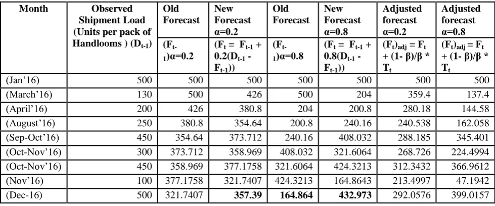
But In order to get which smoothing factor gives better result, comparison between forecasts for α=0.2 and α=0.8 and result shows for α=0.8 is relatively better and accurate forecast. Table 6 shows comparison of the forecasts.

Table 3: Exponential smoothing for trend effects.

Month Observed Shipment Load (Units per pack of

Handlooms ) (Dt-1)

Old Forecast

(Ft-1)

New Forecast (Ft = Ft-1 + .2(Dt-1 -

Ft-1))

Adjusted forecast (Ft)adj = Ft + (1- β)/β * Tt

(Jan‘16) 500 500 500 500

(March‘16) 130 500 426 359.4

(April‘16) 200 426 380.8 380.18

(August‘16) 250 380.8 354.64 340.538

(Sep-Oct‘16) 450 354.64 373.712 388.185

(Oct-Nov‘16) 300 373.712 358.969 368.726

(Oct-Nov‘16) 450 358.969 377.1758 311.533

(Nov‘16) 100 377.1758 321.74065 312.79

(Dec-16) 500 321.74065 357.39 391.69

IV. CONCLUSIONS

(4)

sensitive to real changes in the data. But using Weighted moving averages, given the understanding of the owner of the sales-market head, the weights assigned to the various months of certain period ‗n‘ hugely impacts the forecast value accuracy level. In the given data set, the weights assigned by the stakeholder proves to give best outcome of all forecasts. WMA is the best suited outcome for the dataset. Due to large variation of shipment load in various sequential months, Exponential smoothing technique could not predict better results for simple estimated α=0.2 but with increasing value of

Table 4: A comparative study f forecasts by setting α=0.2 and α=0.8.

Month Observed

Shipment Load (Units per pack of Handlooms ) (Dt-1)

New Forecast α=0.2

New Forecast α=0.8

Adjusted forecast α=0.2

Adjusted forecast α=0.8

(Ft-1)α=0.2 (Ft = Ft-1 + 0.2(Dt-1 - Ft-1))

(Ft-1)α=0.8 (Ft = Ft-1 + 0.8(Dt-1 - Ft-1))

(Ft)adj = Ft + (1- β)/β * Tt

(Jan‘16) 500 500 500 500 500 500 500

(March‘16) 130 500 426 500 204 359.4 137.4

(April‘16) 200 426 380.8 204 200.8 280.18 144.58

(August‘16) 250 380.8 354.64 200.8 240.16 240.538 162.058

(Sep-Oct‘16) 450 354.64 373.712 240.16 408.032 288.185 345.401

(Oct-Nov‘16) 300 373.712 358.969 408.032 321.6064 268.726 224.4994

(Oct-Nov‘16) 450 358.969 377.1758 321.6064 424.3213 312.3432 366.9612

(Nov‘16) 100 377.1758 321.7407 424.3213 164.8643 213.4997 47.1942

(Dec-16) 500 321.7407 357.39 164.864 432.973 292.0576 399.0157

α, a better result is achieved. Setting α=0.8 gives by far closest forecast of the observed shipment load of Lohri (Jan‘17)

as shown in table1. The forecast value Ft is least of all forecasted values and subjected to trend adjustments for α=0.2 but

tends to get stable with increasing value of α. The trend adjustments are affected dramatically due to this level of variation.

REFERENCES

[1] Mathews, B. P., & Diamantopoulos, A. (1986). Managerial intervention in forecasting: An empirical

investigation of forecast manipulation. International Journal of Research in Marketing, 3, 3–10.

[2] Mathews, B. P., & Diamantopoulos, A. (1987). Alternative indicators of forecast revision and improvement.

Marketing Intelligence and Planning, 5, 20–23.

[3] Mathews, B. P., & Diamantopoulos, A. (1989). Judgmental revision of sales forecasts — a longitudinal

extension. Journal of Forecasting, 8, 129–140.

[4] Diamantopoulos, A., & Mathews, B. P. (1989). Factors affecting the nature and effectiveness of subjective

revision in sales forecasting: An empirical study. Managerial and Decision Economics, 10, 51–59.

[5] McNees, S. K. (1990). The role of judgment in macroeconomic forecasting accuracy. International Journal of

Forecasting, 6, 287–299.

[6] Mathews, B. P., & Diamantopoulos, A. (1990). Judgmental revision of sales forecasts — effectiveness of

forecast selection. Journal of Forecasting, 9, 407–415.

[7] Turner, D. S. (1990). The role of judgment in macroeconomic forecasting. Journal of Forecasting, 9, 315–34.

[8] Donihue, M. R. (1993). Evaluating the role judgment plays in forecast accuracy. Journal of Forecasting, 12, 81–

92.

[9] Harvey, N. (1995). Why are judgments less consistent in less predictable task situations? Organizational

Behavior and Human Decision Processes, 63, 247–263.

[10] Lim, J. S., & O‘Connor, M. (1995). Judgmental adjustment of initial forecasts — its effectiveness and biases.

Journal of Behavioral Decision Making, 8, 149–168.

[11] Lim, J. S., & O‘Connor, M. (1996). Judgmental forecasting with time series and causal information.

International Journal of Forecasting, 12, 139–153.

[12] Goodrich, R.L., 2000. The forecast pro methodology. International Journal of Forecasting 16, 533–535.

[13] MacGregor, D. (2001). Decomposition for judgmental forecasting and estimation. In J. S. Armstrong (Ed.),

Principles of forecasting (pp. 107–123). Norwell, MA: Kluwer.

[14] Fader PS and Hardie BGS (2001). Forecasting trial sales of new consumer packaged goods. In: Armstrong J.S.

(ed). Principles of Forecasting: A Handbook for Researchers and Practitioners. Kluwer: Norwell, MA.

[15] Fildes R (2002). Telecommunications demand forecasting—A review. Int J Forecasting 18: 489–522.

[16] Moon, M. A., Mentzer, J. T., & Smith, C. D. (2003). Conducting a sales forecasting audit. International Journal

of Forecasting, 19, 5–25.

[17] Charles C. Holt, ―Author's retrospective on ‗Forecasting seasonals and trends by exponentially weighted moving

(5)

[18] Eaves AHC and Kingsman BG (2004). Forecasting for the ordering and stock-holding of spare parts. J Opl Res

Soc 55: 431–437.

[19] Yaniv, I. (2004). Receiving other people‘s advice: Influence and benefit. Organizational Behavior and Human

Decision Processes, 93, 1–13.

[20] Divakar S, Ratchford BT and Shankar V (2005). CHAN4CAST: A multichannel, multiregion sales forecasting

model and decision support system for consumer packaged goods. Market Sci 24: 334–350.

[21] Gardner, E. S. (2006). Exponential smoothing: The state of the art – Part II. International Journal of Forecasting,

22, 637–666.

[22] Lawrence, M., Goodwin, P., O‘Connor, M., & Onkal, D. (2006). Judgmental forecasting: A review of progress

over the last 25 years. International Journal of Forecasting, 22, 493–518

[23] Fildes R and Goodwin P (2007). Against your better judgment? How organizations can improve their use of

management judgment in forecasting. Interfaces 37: 570–576.

[24] Goodwin, P., Lee, W. Y., Fildes, R., Nikolopoulos, K., & Lawrence, M. (2007). Understanding the use of

forecasting systems: An interpretive study in a supply-chain company. Bath University Management School working paper.

[25] Fildes R, Goodwin P, Lawrence M and Nikolopoulos K (2008). Effective forecasting and judgmental

adjustments: an empirical evaluation and strategies for improvement in supply-chain planning. Int J Forecasting 24.

[26] Fildes, R., Goodwin, P., Lawrence, M., & Nikolopoulos, K. (2009). Effective forecasting and judgmental