Graph Computation Models
Selected Revised Papers from the
Third International Workshop on
Graph Computation Models (GCM 2010)
A Visual Interpreter Semantics for Statecharts
Based on Amalgamated Graph Transformation
Ulrike Golas, Enrico Biermann, Hartmut Ehrig and Claudia Ermel
24 pages
Guest Editors: Rachid Echahed, Annegret Habel, Mohamed Mosbah Managing Editors: Tiziana Margaria, Julia Padberg, Gabriele Taentzer
A Visual Interpreter Semantics for Statecharts
Based on Amalgamated Graph Transformation
Ulrike Golas1, Enrico Biermann2, Hartmut Ehrig2and Claudia Ermel2
1[email protected]Konrad-Zuse-Zentrum f¨ur Informationstechnik Berlin, Germany 2enrico|ehrig|[email protected]Technische Universit¨at Berlin, Germany
Abstract: Several different approaches to define the formal operational semantics
of statecharts have been proposed in the literature, including visual techniques based on graph transformation. These visual approaches either define a compiler seman-tics (translating a concrete statechart into a semantical domain) or they define an interpreter using complex control and helper structures. Existing visual semantics definitions make it difficult to apply the classical theory of graph transformations to analyze behavioral statechart properties due to the complex control structures.
In this paper, we define an interpreter semantics for statecharts based on amalga-mated graph transformation where rule schemes are used to handle an arbitrary number of transitions in orthogonal states in parallel. We build on an extension of the existing theory of amalgamation from binary to multi-amalgamation including nested application conditions to control rule applications for automatic simulation. This is essential for the interpreter semantics of statecharts. The theory of amalga-mation allows us to show termination of the interpreter semantics of well-behaved statecharts, and especially for our running example, a producer-consumer system.
Keywords:operational semantics, statecharts, graph transformation, amalgamation
1
Introduction and Related Work
In [Har87], Harel introduced statecharts by enhancing finite automata by hierarchies, concur-rency, and some communication issues. Over time, many versions with slightly differing fea-tures and semantics have evolved. In the UML specification [OMG09], the semantics of UML state machines is given as a textual description accompanying the syntax, but it is ambiguous and explained essentially by examples. In [Bee02], a structured operational semantics (SOS) for UML statecharts is given based on the preceding definition of a textual syntax for statecharts. The semantics combines Kripke structures and an auxiliary semantics using deduction such that a semantical step is a transition step in the Kripke structure. This semantics is difficult to un-derstand due to its non-visual nature. The same problem arises in [RACH00], where labeled transition systems and algebraic specification techniques are used.
enabled transitions. In [KGKK02], in addition, class and object diagrams are integrated. The approach highly depends on concrete statechart models and is not a general interpreter semantics for statecharts. Moreover, problems arise for nesting hierarchies, because the resulting situation is not fixed but also depends on other current or inactive states. In [GP98], the hierarchies of statecharts are flattened to a low-level graph representing an automaton defining the intended semantics of the statechart model. This is an indirect definition of the semantics, and the resulting transformation rules are model-specific and not applicable to statecharts in general.
In [Var02], Varr´o defines a general interpreter semantics for statecharts. His intention is to separate syntactical and static semantic concepts (like conflicts, priorities etc.) of statecharts from their dynamic operational semantics, which is specified by graph transformation rules. To this end, he uses so-called model transition systems to control the application of the operational rules, which highly depend on additional helper structures encoding activation or conflicts of transitions and states.
Amalgamation is important for graph transformations in order to model synchronized par-allelism of rules with shared subrules and corresponding transformations. For example, it has been applied to applications of parallel graph transformations to communication-based systems [TB94] and to model transformations from BPMN to BPEL [BEE+10]. The concept of amal-gamation was first developed for the synchronization of two rules [BFH87] and then extended to that of an arbitrary number of rules [Tae96] and integrated in the well-known theory ofM -adhesive systems [GEH10]. Using amalgamation for the definition of an operational semantics, the main advantage of our solution is that we do not need helper structures or a complex external control structure to cover the complex statecharts semantics: we define a state transition mainly by one interaction scheme followed by some clean-up rules. Therefore, our model-independent definition based on rule amalgamation is not only visual and intuitive but allows us to show termination and forms a solid basis for applying further graph transformation-based analysis techniques.
The rest of the paper is structured as follows.Section 2gives a brief introduction to our model of statecharts as typed attributed graphs. InSection 3, we review the basic ideas of algebraic graph transformation [EEPT06] and give a short introduction to amalgamated transformation based on [GEH10], which is used for the operational semantics of statecharts inSection 4. Based on the given semantics, we discuss the formal analysis of termination of semantical steps in statecharts. The operational semantics is demonstrated along a sample statechart modeling a producer-consumer system inSection 5. InSection 6, the implementation in our toolHenshinis presented. Finally,Section 7concludes our paper and considers future work directions.
2
Modeling of Statecharts
error call repair prod produced prepare empty full wait consumed arrive finish repair finish exit
next produce[empty] /incbuff fail inc-buff dec-buff next consume [full] /decbuff
Figure 1: Sample statechartProdCons In Figure 1, the sample
statechartProdCons is de-picted modeling a producer-consumer system. When initialized, the system is in the state prod, which has three regions. There, in par-allel a producer, a buffer, and a consumer may act. Parallel substates are
mod-elled in orthogonal regions of a common superstate (separated by dashed lines), which means that while the superstate is active, also exactly one substate from each orthogonal region is ac-tive. The producer alternates between the statesproducedandprepare, where the transition producemodels the actual production activity. It is guarded by a condition that the parallel state emptyis also current, meaning that the buffer is empty and may receive a product, which is then modeled by the actionincbuffdenoted after the/-dash. Similarly to the producer, the buffer alternates between the statesemptyandfull, and the consumer betweenwaitandconsumed. The transitionconsumeis again guarded by the statefulland followed by adecbuff-action emptying the buffer. Two possible events may happen causing a state transition to leave the state prod: the consumer may decide to finish the complete run; or there may be a failure detected after the production leading to theerror-state. After repair, theerror-state can be exited via the correspondingexit-transition and the standard behavior in theprod-state is executed again. For our statechart language, we use typed attributed graphs, which are an extension of typed graphs by attributes [EEPT06]. We do not give details here, but use an intuitive approach, where the attributes of a node are given in a class diagram-like style. For the values of attributes in the rules we can also use variables. SM
name:String R P E name:String T S name:String isInitial:Bool isFinal:Bool TE name:String A name:String G
0..1
0..1 0..1 1
1 1
1
0..1
1 0..1
1
1 1..n
1..n
region behavior current new regions states trigger action guard begin end condition next sub
Figure 2: Type graphT GSCfor statecharts The type graphT GSCis given
in Figure 2. We use multiplic-ities to denote some constraints directly in the type graph. To obtain valid statechart models, additional constraints are de-fined inFigure 3. We use nested conditions, which are defined explicitely inSection 3and can be intuitively understood as the
requirement to find occurrences of the morphism’s domain and codomain in the target object leading to commuting diagrams. Note that iA defines the unique morphism from an initial ob-jectI to some object A. Each diagram consists of exactly one statemachineSM(constraintc1) containing one or more orthogonal regionsR. A region contains statesS, where state names are unique within one region. A state may again contain one or more regions. Constraintc2
final states cannot contain regions (constraint c3). Note that the edge typesubis only
neces-sary to compute all substates of a state, which we need for the definition of the semantics. This relation is computed in the beginning using thestates- andregions-edges.
A transitionTbegins and ends at a state, is triggered by an eventE, and may be restricted by a guardGand followed by an actionA. A guard has one or more states as conditions. There is a special event with attribute valuename="exit"which is reserved for exiting a state after the completion of all its orthogonal regions, which cannot have a guard condition (constraintc4).
Moreover, final states cannot be the beginning of a transition and their name attribute has to be set toname="final"(constraint c5). In addition, transitions cannot link states in different
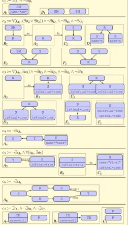
c1:=∃iA1∧ ¬∃iB1 SM
name="sm"
A1 B1 SM SM
c2:=∀(iA2,(∃a2∨ ∃b2))∧ ¬∃iD2∧ ¬∃iE2∧ ¬∃iF2 SM R B2 R A2 S R C2 SM S R E2 S S R F2 S name=x S name=x R D2
c3:=∀(iA3,∃a3)∧ ¬∃iC3∧ ¬∃iD3∧ ¬∃iE3∧ ¬∃iF3 R A3 S isInitial=true R B3 S isInitial=true S isInitial=true R C3 S isFinal=true S isFinal=true R D3 S isFinal=true R E3 S isInitial=true isFinal=true F3
c4:=¬∃iA4
G T E
name="exit"
A4
c5:=¬∃iA5∧ ∀(iB5,∃a5)
T S isFinal=true A5 S isFinal=true B5 S name="final" isFinal=true C5
c6:=¬∃iA6
S R R S S T A6
c7:=∃iA7∧ ¬∃iB7∧ ¬∃iC7 TE name=null P A7 P P C7 TE name=null TE B7 begin end begin
a2 b2
a3
a5
Figure 3: Constraints limiting the valid statecharts orthogonal regions (constraintc6),
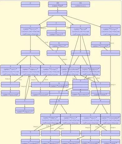
P TE name=null SM name="sm" R S name="error" isInitial=false isFinal=false S name="prod" isInitial=true isFinal=false T E name="exit" S name="final" isInitial=false isFinal=true R S name="call" isInitial=true isFinal=false S name="repair" isInitial=false isFinal=false S name="final" isInitial=false isFinal=true T E name="arrive" T E name="finish" T E name="repair" T E name="fail" R S name="produced" isInitial=true isFinal=false T E name="next" T E name="produce" G A name="incbuff" S name="prepare" isInitial=false isFinal=false R S name="empty" isInitial=true isFinal=false S name="full" isInitial=false isFinal=false R S name="wait" isInitial=true isFinal=false S name="consumed" isInitial=false isFinal=false T E name="next" T E name="consume" G A name="decbuff" T E name="decbuff" T E name="incbuff" T E name="finish" end begin begin end begin
end begin end
begin end begin end begin end begin end begin end begin end begin end begin end
Figure 4: StatechartProdConsin abstract syntax
In Figure 4, the sample statechart ProdConsfrom Figure 1is depicted in abstract syntax. NodesPandTEare added, which have to exist for a valid statechart model but are not visible in the concrete syntax. For simulating statechart runs, the event queue of the statechart (consisting of only one default element namednullinFigure 4) can be filled by events to be processed (see
Since edges of typessub,behavior,current, andnextonly belong to the semantics but not to the syntax of statecharts, we leave them out for the definition of the language of statecharts. All attributed graphs typed over this reduced type graphT GSC,Syn satisfying all the constraints are valid statecharts.
Definition 1 (Language V LSC) Define the syntax type graph T GSC,Syn = T GSC\{sub,
behavior,current,next} based on the type graph T GSC in Figure 2. The language V LSC consists of all typed attributed graphs respecting the type graphT GSC,Synand the constraints in
Figure 3, i. e.V LSC={(G,type)|type:G→T GSC,Syn,G|=c1∧. . .∧c7}.
3
Introduction to Amalgamated Graph Transformation
In this section, we review the basic ideas of algebraic graph transformation [EEPT06] and give a short introduction into amalgamated transformation based on [GEH10], to be used for the interpreter semantics of statecharts inSection 4.
A graph grammar GG= (RS,SG) consists of a set of rulesRS and a start graphSG. A rule
p= (L←−l K−→r R,ac)consists of a left-hand sideL, an interfaceK, a right-hand sideR, two
injective graph morphismsL←−l KandK−→r R, and an application conditionaconL. Applying a rulepto a graphGmeans to find a matchmofLinG, given by a graph morphismm:L→G
which satisfies the application conditionac, and to replace this matched partm(L)by the corre-sponding right-hand sideRof the rule. ByG=p,⇒m H, we denote the direct graph transformation where rule p is applied to Gwith match m leading to the resultH. The formal construction of a direct transformation is a double-pushout (DPO) as shown in the diagram with pushouts
L K R
G D H
ac l r
m (PO1) (PO2)
(PO1)and(PO2)in the category of graphs. The graphDis
the intermediate graph after removingm(L), andH is con-structed as gluing ofDand Ralong K. A graph transfor-mation is a sequence of direct transfortransfor-mations, denoted by
G=∗⇒H, and the graph languageL(GG)of graph grammar
GGis the setL(GG) ={G| SG=∗⇒G}of all graphs derivable fromSG.
An important concept of algebraic graph transformation is parallel and sequential indepen-dence of graph transformation steps leading to the Local Church–Rosser and Parallelism Theo-rem [Roz97], where parallel independent stepsGp=1,⇒m1G1andG
p2,m2
=⇒G2lead to a parallel
trans-formationGp1=+p⇒2,mH based on a parallel rule p1+p2. If p1 and p2 share a common subrule
p0, the amalgamation theorem in [BFH87] shows that a pair of “amalgamable” transformations
G(p=i⇒,mi)Gi(i=1,2)leads to an amalgamated transformationG
˜
p,m˜
=⇒Hvia the amalgamated rule ˜
p=p1+p0p2constructed as gluing ofp1 andp2along p0. The concept of amalgamable
trans-formations is a weak version of parallel independence, with independence outside the subrule match, and amalgamation can be considered as a kind of “synchronized parallelism”.
For the interpreter semantics of statecharts we need an extension of amalgamation in [BFH87] w.r.t. three aspects: first, we need a family of rules p1, . . . ,pn with a common subrule p0 for
In the following, we formulate the extended amalgamation concept for a general notion of graphs and application conditions, wheregeneral graphs are objects in a weak adhesive HLR category [EEPT06] andgeneral application conditionsare nested application conditions [HP09], including positive and negative ones and their combinations by logic operators. For readers not familiar with weak adhesive HLR categories and nested application conditions, it is sufficient to think of rules based on graphs and (typed) attributed graphs with positive and/or negative application conditions (see [EEPT06] for more details).
A matchm:L→Gsatisfies a positive (negative) condition of the form∃a(¬∃a)fora:L→N
if there is a (no) injectiveq:N→Gwithq◦a=m. More general,m:L→Gsatisfies a nested condition of the form∃(a,acN)onLwith conditionacN onNif there is an injectiveq:N→G withq◦a=mandqsatisfiesacN. Note that∀(a,acN)is denoted as¬∃(a,¬acN)(see application conditions inFigure 9andFigure 10).
L L0
G
ac t Shift(t,ac)
m = m0
An important concept is the shift of ac on L along a morphism t:L→ L0 s.t. for all m0◦t :L→G, m0
satisfies Shift(t,ac) if and only if m=m0◦t:L→G
satisfiesac[EHL10].
Based on [GEH10], we are now able to introduce amalgamated rules and transformations with a common subrulep0of p1, . . . ,pn. A kernel morphism describes how the subrule is embedded
into the larger rules.
L0 K0 R0
Li Ki Ri
l0 r0
si,L (1i) si,K (2i) si,R
Definition 2 (Kernel morphism). Given rules pi = (Li
li
←−
Ki ri
−→Ri,aci)for i=0, . . . ,n, akernel morphismsi:p0→pi
consists of morphisms si,L:L0→Li, si,K :K0→Ki, and si,R:
R0→ Ri such that in the diagram on the right (1i) and(2i)
are pullbacks and(1i) has a pushout complement for si,L◦l0,
i.e. si,Lsatisfies the gluing condition w.r.t. l0. The pullbacks (1i) and(2i)mean that K0 is the
intersection of Ki with L0and also of Kiwith R0.
p0 p˜
pi t0
si = ti
Definition 3 (Amalgamated rule and transformation). Given rules pi =
(Li li
←−Ki ri
−→Ri,aci)for i=0, ..,n with kernel morphisms si:p0→pi (i=
1, . . . ,n), then the amalgamated rulep˜= (L˜←−K˜−→R˜,ac˜ )of p1, . . . ,pnvia
p0 is constructed as the componentwise gluing of p1, . . . ,pnalong p0, where
˜
ac is the conjunction of Shift(ti,L,aci). L is the gluing of L˜ 1, . . . ,Ln with shared L0 leading to
ti,L:Li →L. Similar gluing constructions lead to˜ K and˜ R and we obtain kernel morphisms˜
ti:pi→p and t˜ i◦si=t0for i=1, . . . ,n. We call p0kernel rule, and p1, . . . ,pn multi rules. An
amalgamated transformation G=p⇒˜ H is a transformation via the amalgamated rulep.˜
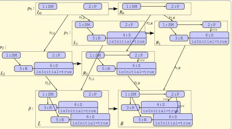
Example 1 (Amalgamated rule construction) We construct an amalgamated rule for the ini-tialization of a statemachine with two orthogonal regions. A pointer has to be linked to the statemachine and to the initial states of both the statemachine’s regions. Rules are depicted in a
compact notation where we do not show the interfaceK. It can be inferred by the intersection
L∩R. The mappings are given as numberings for nodes and can be inferred for edges. The
kernel rule p0 inFigure 5models the linking of the pointer to the statemachine. We have two
p0: 1:SM 2:P
L0
1:SM 2:P
R0
p1:
1:SM 2:P
3:R 4:S
isInitial=true
L1
1:SM 2:P
3:R 4:S
isInitial=true
R1
p2:
1:SM 2:P
5:R 6:S
isInitial=true
L2
1:SM 2:P
5:R 6:S
isInitial=true
R2
˜
p:
1:SM 2:P
3:R 4:S
isInitial=true
5:R 6:S
isInitial=true ˜
L
1:SM 2:P
3:R 4:S
isInitial=true
5:R 6:S
isInitial=true ˜
R
s1,L s1,R
s2,L
s2,R
t1,L
t1,R
t2,L t2,R
new
new
new new
Figure 5: Construction of amalgamated rule
regions. In the amalgamated rule p˜, the common subaction (linking the pointer to the
statema-chine) is represented only once since the multi-rulesp1andp2have been glued at the kernel rule
p0. The kernel morphisms areti:pi→p˜fori=1,2.
Given a bundle of direct transformations G=pi⇒,mi Gi (i=1, ..,n), where p0 is a subrule of
pi, we want to analyze whether the amalgamated rule ˜pis applicable toGcombining all direct transformations. This is possible if they aremulti-amalgamable, i.e. the matches agree onp0and are parallel independent outside. This concept of multi-amalgamability is a direct generalization of amalgamability in [BFH87] and leads to the following theorem [GEH10].
Theorem 1 (Multi-amalgamation) Given rules p0, . . . ,pn, where p0 is a subrule of pi, and
multi-amalgamable direct transformations G=pi⇒,miGi(i=1, . . . ,n), then there is an amalgamated
transformation G=p˜⇒,m˜ H.
Proof Idea: Using the properties of the multi-amalgamable bundle, we can show that ˜mwith ˜
m◦ti,L=mi induced by the colimit is a valid match for the amalgamated rule ˜p leading to the amalgamated transformation because the componentwise gluing is a colimit construction. For an extended proof idea see Thm. 2 in [GEH10], the complete proof can be found in [Gol11].
Definition 4(Interaction scheme) A kernel rule p0 and a set of multi rules{p1, . . . ,pk}with kernel morphismssi:p0→piform an interaction schemeis={s1, . . . ,sk}.
Given an interaction scheme, we want to apply as many rules pj as often as possible over a certain match of the kernel rule p0. In the following, we consider maximal weakly disjoint
matchings, where we require the matchings of the multi rules not only to be multi-amalgamable,
but also disjoint up to the match of the kernel rule, and maximal in the sense that no more valid matches for any multi rule in the interaction scheme can be found.
L0 L0i
L0` G
si,L
s`,L mi
m` (Pi`)
Definition 5(Maximal weakly disjoint matching). Given an interaction
scheme is={s1, . . . ,sk}and a tuple of matchings m= (mi:L0i→G)with
i=1, . . . ,n, where each p0icorresponds to some pj for j≤k, with
trans-formations Gp
0
i,mi
=⇒Gi, then m forms amaximal weakly disjoint matchingif
the bundle Gp
0
i,mi
=⇒Giis multi-amalgamable, the square(Pi`)is a pullback for all i6=`∈ {1, . . . ,n}, and for any rule pjno other match m0:Lj→G can be found such that((mi),m0)fulfills this
prop-erty.
Note that different matches may use the same rule pj. The pullback requirement already implies the existence of the morphisms to show that the matches are parallel independent outside the kernel match. Only the property for the application conditions has to be checked in addition.
Proposition 1 Given an object G, a bundle of kernel morphisms s= (s1, . . . ,sn), and matches
m1, . . . ,mn leading to a bundle of direct transformations G=
pi,mi
==⇒ Gi such that mi◦si,L=m0
and square (Pi`) is a pullback for all i6=` then the bundle G=
pi,mi
==⇒ Gi is s-amalgamable for
transformations without application conditions.
Proof. By construction, the matchesmi agree on the matchm0of the kernel rule. It remains to
be shown that they are parallel independent outside the kernel match.
K0
L0
Ki
Li
P
Lj
Di
G
Ki Ri
Di Gi
Li
G
l0
si,K
p
sj,L
si,L
li
ki
ˆ
f
ˆ
m
mj
fi mi
fi
li
mi
ri
ki
gi
ni
(20i) (21i)
Given the transfor-mations G=pi,mi
==⇒ Gi
with pushouts (20i)
and (21i), consider the following cube, where the bottom face is pushout (20i), the back right face is a
pullback by definition, and the front right face is pullback(Pi j). Now construct the pullback of fiandmj as the front left face, and frommj◦sj,L◦l0=mi◦si,L◦l0=mi◦li◦si,K= fi◦ki◦si,K we obtain a morphismpwith ˆf◦p=sj,L◦l0and ˆm◦p=ki◦si,K.
With this characterization of maximal weakly independent matches we obtain the following algorithm for their computation.
Algorithm 1(Maximal weakly disjoint matching). Given an object G and an interaction scheme
is={s1, . . . ,sk}, a maximal weakly disjoint matching m= (m0,m1, . . . ,mn)can be computed as
follows:
1. Set i=0. Choose a kernel matching m0:L0→G such that G=
p0,m0
===⇒G0 is a valid
trans-formation.
2. As long as possible: Increase i, choose a multi rule pˆi=pjwith j∈ {1, . . . ,k}, and find a
match mi:Lj→G such that mi◦sj,L=m0, G=
pj,mi
==⇒Giis a valid transformation, mi6=m`, the square(Pi`)is a pullback, and pˆ` is applicable to Givia the extension of m`to Gifor
all`=1, . . . ,i−1, i.e. the application conditionacˆ`is satisfied for this extended match.
3. If no more valid matches for any rule in the interaction scheme can be found, return m= (m0,m1, . . . ,mn).
Note, that we may find different maximal weakly disjoint matchings for a given interaction scheme, which may even lead to the same bundle of kernel morphisms. For a fixed maximal
weakly disjoint match we can applyTheorem 1leading to an amalgamated transformationG p˜
0,m˜
=⇒
H, where ˜p0is the amalgamated rule ofp01, . . . ,p0nvia p0.
Given a set IS of interaction schemes is and a start graph SG, we obtain an amalgamated graph grammar with amalgamated transformations via maximal matchings, defined by maximal weakly disjoint matchings of the corresponding multi rules.
Definition 6(Amalgamated graph grammar) Anamalgamated graph grammar AGG= (IS,SG)
consists of a setISof interaction schemes and a start graphSG. Thelanguage L(AGG)ofAGG
is defined byL(AGG) ={G| ∃amalgamated transformationSG=⇒∗ Gvia maximal matchings}.
4
An Interpreter Semantics for Statecharts
The semantics of statecharts is modeled by amalgamated transformations, where one step in the semantics is modeled by several applications of interaction schemes. The main part of a state transition can be modeled by a single interaction scheme, but some additional rules are necessary to remove and add the proper pointers from and to hierarchical states. For the application of an interaction scheme we use maximal weakly disjoint matchings.
general for well-behaved statecharts, where we forbid cycles in the dependencies of actions and events.
Definition 7(Well-behaved statecharts) For a given statechart model, theaction-event graph
has as nodes all event names and an edge(n1,n2)if an event with name n1 triggers an action namedn2.
A statechart is calledwell-behavedif it is finite, has an acyclic state hierarchy, and its action-event graph is acyclic.
Example2 An example of a well-behaved statechart is our statechart model inFigure 1. It is
finite, has an acyclic state hierarchy, and its action-event graph is shown inFigure 6. This graph
is acyclic, since the only action-event dependencies in our statechart occur betweenproduce
triggeringincbuffandconsumetriggeringdecbuff.
arrive repair fail produce incbuff
next finish exit consume decbuff
Figure 6: The action-event graph of our statechart example
The semantics of our statecharts is modeled by amalgamated transformations, but we apply the rules in a more restricted way, meaning that one step in the semantics is modeled by several applications of interaction schemes. We assume to have a finite statechart with a finite event queue where all trigger elements are already given in the diagram as an initial event queue.
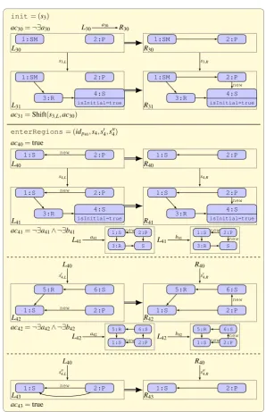
For theinitialization step, we compute all substates of all states by applying the rulessetSub andtransSubinFigure 7as long as possible. Then, the interaction schemeinitis applied followed by the interaction scheme enterRegions applied as long as possible, which are depicted inFigure 8. Withinit, the pointer is associated to the statemachine and all initial states of the statemachine’s regions. The interaction schemeenterRegionshandles the nesting and sets the current pointer also to the initial states contained in an active state. When applied as long as possible, this means that all substates are handled. Note that not all initial substates become
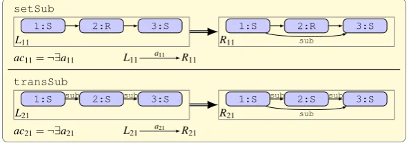
setSub
1:S 2:R 3:S
L11
1:S 2:R 3:S
R11
ac11=¬∃a11 L11 R11
transSub
1:S 2:S 3:S
L21
1:S 2:S 3:S
R21
ac21=¬∃a21 L21 R21
a11
sub
a21
sub sub sub sub
sub
init= (s3)
1:SM 2:P
L30
1:SM 2:P
R30
1:SM 2:P
3:R 4:S
isInitial=true
L31
1:SM 2:P
3:R 4:S
isInitial=true
R31 ac30=¬∃a30 L30 R30
ac31=Shift(s3,L,ac30)
enterRegions= (idp40,s4,s
0
4,s004)
1:S 2:P
L40
1:S 2:P
R40
1:S 2:P
3:R 4:S
isInitial=true
L41
1:S 2:P
3:R 4:S
isInitial=true
R41 ac40=true
ac41=¬∃a41∧ ¬∃b41 L41
1:S 2:P
3:R S L41
1:S 2:P
3:R S
L40 R40
1:S 2:P
5:R 6:S
L42
1:S 2:P
5:R 6:S
R42 ac42=¬∃a42∧ ¬∃b42
L42
1:S 2:P 5:R 6:S
L42
1:S 2:P 5:R 6:S
L40 R40
1:S 2:P
L43
1:S 2:P
R43 ac43=true
a42 b42
new new
new
new
a41 b41
new new
new
new
new
a30
s3,L s3,R
s4,L s4,R
s04,L s
0 4,R
s00
4,L s
00 4,R
new
new
new
new
Figure 8: The interaction schemesinitandenterRegions
active, but only those which are contained in a hierarchy of nested initial states. The interaction schemeenterRegionsalso contains the identical kernel morphismidp40:p40→p40. Using
The application of the rules setSubandtransSubterminates because there could be at most onesub-edge between each pair of states due to the application conditions. Since no new states are created, these rules can only be applied finitely often.
The initialization step (applying initonce andenterRegionsas long as possible) termi-nates because the application of the interaction schemeenterRegionsterminates: each appli-cation ofenterRegionsreplaces onenew-edge with acurrent-edge. The multi rules p41
andp42create newnew-edges on the next lower and upper levels of a hierarchical state, but if the
state hierarchy is acyclic this interaction scheme is only applicable a finite number of times. The same holds for the multi rule p43 which deletes double edges, since the number ofcurrent
-andnew-edges is decreased. Thus, the transformation terminates.
Proposition 2(Termination of initialization step) For well-behaved statecharts, the
initializa-tion step terminates.
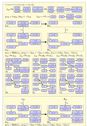
A state transition representing a semantical step, i. e. switching from one state to another, is done by the application of the interaction scheme transitionStep shown in Figure 9
followed by the interaction schemesenterRegions!,leaveState1!,leaveState2!, and leaveRegions! given in Figure 8, 10, and 11 in this order, where ! means that the corresponding interaction scheme is applied as long as possible.
For such a semantical step, the first trigger element (or one of the first if more than one action of different orthogonal substates may occur next) is chosen and deleted, while the corresponding state transitions are executed. The application conditionac50ensures thatexit-trigger elements
are handled with priority, because the rule is only applicable if for any existingexit-trigger el-ement (∀a50) this is not a start element in the queue, i.e. it has a predecessor (∃b50). Moreover,
it ensures that the chosen trigger element is a starting one, i.e. has no predecessor (¬∃c50). Note
that a transition triggered by its trigger element is active if the state it begins at is active, its guard condition state is active, and it has no active substate where a transition triggered by the same event is active. These restrictions are handled by the application conditionsac51andac52.
More-over, if an action is provoked, this has to be added as one of the first next trigger elements. The two multi rules oftransitionStep handle the state transition with and without action, re-spectively. The application conditionac52is not shown explicitly, but the morphismsa52, . . . ,f52
are similar toa51, . . . ,f51except that all objects contain in addition the node8:A.
The interaction schemesleaveState1,leaveState2, andleaveRegionshandle the correct selection of the active states. When for a yet active state with regions, by state transitions all states in one of its regions are no longer active, also this superstate is no longer active, which is described byleaveState1. The interaction schemeleaveState2handles the case that, when a state become inactive by a state transition, also all its substates become inactive. If for a state with orthogonal regions the final state in each region is reached then these final states become inactive, and if the superstate has an exit-transition it is added as the next trigger element. This is handled byleaveRegions.
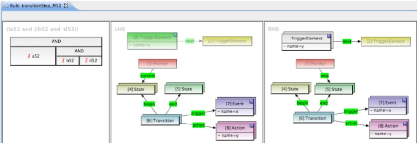
transitionStep= (s5,s05) L50 1:P 2:TE name=x TE name="exit" 3:TE 1:P 3:TE TE TE name="exit" 2:TE name=x
ac50=∀(a50,∃b50)∧ ¬∃c50 L50 1:P TE 2:TE name=x 3:TE 1:P 2:TE name=x 3:TE L50 1:P 3:TE R50 1:P 2:TE name=x 3:TE 4:S 5:T 6:S 7:E name=x L51 1:P 3:TE 4:S 5:T 6:S 7:E name=x R51
ac51=Shift(s5,L,ac50)∧ ¬∃g51∧ ¬∃a51∧ ∀(b51,∃c51)∧ ∀(d51,∃(e51,¬∃f51)) L51 L52 L51 A5 L51 B5 C5 L51 D5 E5 F5
1:P 2:TE name="exit" 3:TE 4:S 5:T S 6:S 7:E name="exit" A5 1:P 2:TE name=x 3:TE 4:S 5:T 6:S 7:E name=x G S B5 1:P 2:TE name=x 3:TE 4:S 5:T 6:S 7:E name=x G S C5 1:P 2:TE name=x 3:TE 4:S 5:T 6:S T E name=x 7:E name=x S D5 1:P 2:TE name=x 3:TE 4:S 5:T 6:S T E name=x 7:E name=x S G S E5 1:P 2:TE name=x 3:TE 4:S 5:T 6:S T E name=x 7:E name=x S G S F5
L50 R50
1:P 2:TE name=x 8:A name=y 3:TE 4:S 5:T 6:S 7:E name=x L52 TE name=y 1:P 3:TE 4:S 5:T 6:S 7:E name=x 8:A name=y R52
ac52=Shift(s05,L,ac50)∧ ¬∃a52∧ ∀(b52,∃c52)∧ ∀(d52,∃(e52,¬∃f52))
s5,L s5,R
a50 b50
c50
g51 a51 b51 c51 d51 e51 f51
begin end new begin end begin end begin end begin end begin end begin begin end begin begin end begin s0
5,L s05,R
begin
end
new
begin
end
Figure 9: The interaction schemetransitionStep
p81 of the interaction schemeleaveRegionsreduce the number of active states in the
state-chart by deleting at least onecurrent-edge. The application of the second multi rule p82 of
the interaction schemeleaveRegionsprevents another match for itself because it creates the situation forbidden by its application conditionac82. It follows that the application of each of
leaveState1= (idp60) ac60=∃(a60,¬∃b60) L60
1:S 2:P
R
1:S 2:P
R S
1:S 2:P
L60
1:S 2:P
R60
leaveState2= (s7)
ac70=¬∃a70 L70 1:S 2:P
1:S 2:P
L70
1:S 2:P
R70
1:S 3:S 2:P
L71
1:S 3:S 2:P
R71 ac71=Shift(s7,L,ac70)
a70
s7,L s7,R
a60 b60
Figure 10: The interaction schemesleaveState1andleaveState2
leaveRegions= (s8,s08)
ac80=∀(a80,∃b80)∧ ¬∃c80∧ ¬∃d80 L80
1:S 2:P TE 3:TE
L80
1:S 2:P 3:TE
R S
isFinal=true
1:S 2:P 3:TE
R S
isFinal=true
L80
1:S 2:P 3:TE
S isFinal=false
1:S 2:P 3:TE
L80
1:S 2:P 3:TE
R80
1:S 2:P 3:TE
4:S
L81
1:S 2:P 3:TE
4:S
R81 ac81=Shift(s8,L,ac80)
L80 R80
1:S 2:P 3:TE
4:T 5:E
name="exit"
L82
1:S 2:P 3:TE
4:T 5:E
name="exit"
TE
name="exit"
R82
ac82=Shift(s08,L,ac80)∧ ¬∃a82 L82
1:S 2:P 3:TE name="exit" 4:T 5:E
name="exit" begin
a82
s8,L s8,R
d80
c80
b80
a80
begin begin
s0
8,L s
0 8,R
Proposition 3(Termination of semantical steps) Given a well-behaved statechart, each seman-tical step terminates.
Combining all the rules as explained above leads to the semantics of statecharts.
Definition 8 (Statechart semantics) The operational semantics of statecharts consists of one
initialization step followed by as many as possible semantical steps defined as follows:
• Initialization step. For a statechart modelM∈V LSC (seeDefinition 1) we obtain a model
Minitial by applying the sequencesetSub!,transSub!,init,enterRegions! to
M.
• Semantical step. Consider a modelM1 with M1 obtained by a finite number of
seman-tical steps from a model Minitial for some M∈V LSC, then a semantical step from M1
toM2 is computed by applying the sequencetransitionStep, enterRegions!,
leaveState1!,leaveState2!,leaveRegions!toM1.
Moreover, combining our termination results we can conclude the termination of the state-charts semantics for well-behaved statestate-charts.
Theorem 2 (Termination of interpreter semantics) For well-behaved statecharts with finite
event queue, the interpreter semantics terminates.
Proof. According toProposition 2andProposition 3, each initialization step and each semanti-cal step terminates. Moreover, each semantisemanti-cal step consumes an event from the event queue. If it triggers an action, the acyclic action-event graph ensures that there are only chains of events triggering actions, but no cycles, such that after the execution of this chain the number of ele-ments in the event queue actually decreases. Thus, after finitely many semantical steps the event queue is empty and the operational semantics terminates.
5
Application to the Running Example
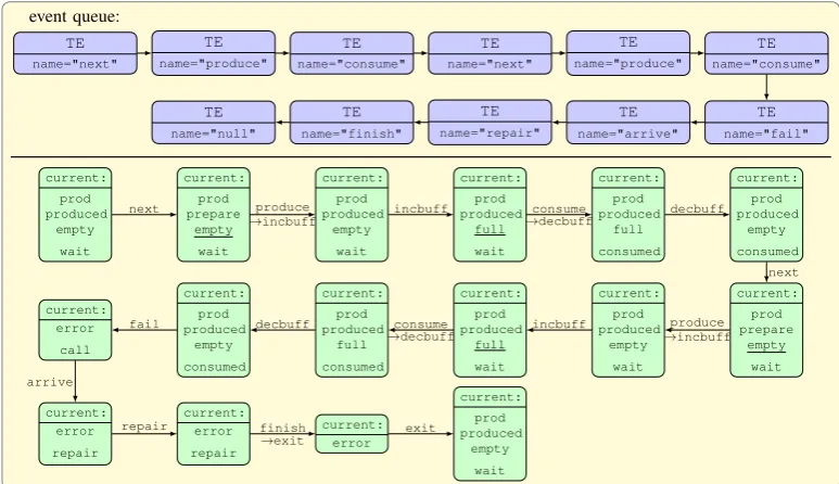
We now consider an initialization and a semantical step in our statechart example fromFigure 1. In the top ofFigure 12, we show the incoming event queue as needed for our system run to be processed. Note that the actions that are triggered by state transitions do not occur here because they are started internally, while the other events have to be supplied from the outside. Thus, the internal events are supplied by the semantical rules themselves, while the external ones have to be given. For simplicity, we assume that the complete external event queue is given in advance, but the events could also appear one after the other using some additional rule that appends an event at the end of the queue. In the bottom ofFigure 12, the current states and their corresponding state transitions are depicted. We want to simulate these semantical steps now using the rules for the semantics applied to the statechart in abstract syntax inFigure 4, extended by the event queue fromFigure 12.
current: prod produced empty wait current: prod prepare empty wait current: prod produced empty wait current: prod produced full wait current: prod produced full consumed current: prod produced empty consumed current: prod prepare empty wait current: prod produced empty wait current: prod produced full wait current: prod produced full consumed current: prod produced empty consumed current: error call current: error repair current: error repair current: error current: prod produced empty wait event queue: TE name="next" TE name="produce" TE name="consume" TE name="next" TE name="produce" TE name="consume" TE name="null" TE name="finish" TE name="repair" TE name="arrive" TE name="fail" next produce →incbuff incbuff consume →decbuff decbuff next produce →incbuff incbuff consume →decbuff decbuff fail arrive repair finish →exit exit
Figure 12: Event queue and state transitions
the interaction scheme init from Figure 8followed by the application of enterRegions as long as possible. Withinit, we connect the state machine and the pointer node, and in addition set the pointer to the prod-state using a new-edge. Now the only available kernel match forenterRegionsis the match mapping node1to theprod-state, and with maximal matchings we obtain the bundle of kernel morphisms(idp40,s4,s4,s4), where the node4inL41
is mapped to the statesproduced,empty, andwait, respectively. After the application of the corresponding amalgamated rule, the current pointer is now connected to the state machine and the stateprod, and vianew-edges to the statesproduced, empty, andwait. Further applications ofenterRegions using these three states for the kernel matches, respectively, lead to the bundle(idp40)thus changing thenew-edges tocurrent-edges by its application.
error call repair prod produced prepare empty full wait consumed arrive finish repair finish exit
next produce[empty] /incbuff fail inc-buff dec-buff next consume [full] /decbuff
Figure 13: The statechart after the initialization step As a result, the statesprod,
produced, empty, and wait are current, which is the initial situation for the statemachine as shown in Figure 13, where the current states are marked by thicker lines. We do not find additional matches forenterRegions, as we
For a state transition, the interaction schemetransitionStepinFigure 9is applied, fol-lowed by the interaction schemesenterRegions!,leaveState1!,leaveState2!, and leaveRegions!given inFigure 8,10, and11.
For the initial situation, the kernel rule p50inFigure 9has to be matched such that the node
2is mapped to the first trigger elementnextand the node3toproduce, otherwise the ap-plication condition of the rule p50would be violated. For the multi rules, there are two events
with the name next, but since the state consumedis not current, only one match for L51
is found mapping the nodes 4 to the current state producedand 6 to the state prepare. All application conditions are fulfilled, since this transition does not have a guard or action, and the stateproduceddoes not have any substates. Thus, the application of the bundle(s5)
deletes the first trigger elementnext, which is done by the kernel rule, and redirects the current pointer fromproducedtopreparevia anew-edge. An application of the interaction scheme enterRegionsusing the bundle(idp40) changes thisnew-edge to acurrent-edge. Since
we do not find further matches for L40, L60, L71, L81, and L82, the other interaction schemes cannot be applied. This means that the statesprod, prepare, empty, andwait are now the current states, which is the situation after the state transition triggered bynextas shown in
Figure 12.
For the next match of the kernel rule p50, the node 2is mapped to the new next trigger
ele-mentproduceand3is mapped toconsume. Since the transition producehas an action, we cannot apply the multi rule p51butp52 has a valid match. In particular, the application con-dition is fulfilled because the guard concon-dition state emptyis current and the state prepare does not have any substates. Thus, the bundle(s05) leads to the deletion of the trigger element produce, the current pointer is redirected from prepare to produced, and a new trig-ger elementincbuffis inserted with anext-edge to the trigger elementconsume. Again, enterRegionschanges the new- to acurrent-edge and we do not find further matches forL40,L60,L71,L81, andL82. This means that now the statesprod,produced,empty, and
waitare current.
We can process our trigger element queue step by step retracing the state transitions by the application of the rules. We do not explain all steps explicitly, but skip until after the last decbuff-trigger element, which leads to the current statesprod, produced, empty, and consumed.
The next match of the kernel rule p50 maps the nodes 2to the trigger element fail and
3toarrive. The only match for the multi rules maps the nodes 4and6inL51to the states producedanderror, respectively. Since the application condition is fulfilled, the application of the bundle (s5) leads to the deletion of the trigger element fail, and the current pointer
is redirected from produced to error. Now we find a match for the interaction scheme enterRegionsmapping the node1to the stateerrorand4to the state call. Thus the application of the bundle(idp40,s4)adds a new pointer to the statecall, which is then changed
fromnew tocurrent. Afterwards, we find a match forleaveState1, where the kernel rule match maps the node1to the stateprod. The application condition is fulfilled because there is a region - the one for the producer - where no state is current. Thus, thecurrent -edge to prod is deleted. No more matches forL60 can be found, but there are two different matches for the multi rule p71ofleaveState2matching the node3to the statesemptyand
current pointer for the statesemptyandconsumed. No more matches forL71,L81, andL82can
be found. Altogether, the stateserrorandcallare current now. This is exactly the situation as described inFigure 12after the state transition triggered by thefail-event.
Now we skip again two more trigger elements leading to the remaining trigger element queue finish → null and the current stateserror andrepair. The kernel rule p50 is now matched to these two trigger elements, and the application of the bundle(s5)deletes the trigger
elementfinishand redirects the current pointer fromrepairtofinal, the final state within the error-state. With enterRegions, the corresponding new-edge is set to current. No matches for L60 and L71 can be found, but we find a match for the interaction scheme
leaveRegions, where the kernel rule is matched such that the node1is mapped to the state errorand3is mapped to thenull-trigger element. The application condition is fulfilled be-cause all current substates oferrorare final states - actually, there is only the one - andnull is the first trigger element in the queue. Now there is a match forL81 mapping the node4to
the statefinaland a match forL82 mapping the nodes4and5to the transition and the event between the stated errorandprod. After the application of the bundle (s8,s08), the current
pointer is deleted from the final-state, and a new exit-trigger element is inserted before thenull-trigger element. No more matches forL81 andL82 can be found, thus only the state erroris current. A last application of the interaction schemetransitionStepfollowed by enterRegionsleads back to the initial situation and completes our example, since the event queue is empty except for the default elementnull.
According to Thm.2, the simulation of our example terminates because our statechart is
well-behaved and the event queue is finite.
6
Implementation
Recently, we have extended our toolHenshin1by visual editors for amalgamated rules and ap-plication conditions [BESW10]. Henshinis an Eclipse plug-in supporting visual modeling and execution of EMF model transformations, i.e. transformations of models conforming to a meta-model given in the EMF Ecore format. The transformation approach we use in our tool is based on graph transformation concepts which are lifted to EMF model transformation by also taking containment relations in meta-models into account [ABJ+10].
The recent extensions of Henshin enable us to validate the model of the visual interpreter semantics presented in this paper. The startgraph of our statechart interpreter is modeled in
Henshinas an EMF instance (seeFigure 14).
For simulation, Henshin supports the definition of control structures (called transformation units) for rules, such as“apply rule r1once, and then the rules from the set{r1,r2}in arbitrary
order and as long as possible”. Transformation units may be nested, the atomic unit being a rule.
The main transformation unit for the statechart simulation is shown in Figure 15. Here, the initialization step is executed by applying the subunitinitStatechart(see right part ofFigure 15). This step is realized by a sequence of units inserting at first the auxiliary edges of the type
sub in the statechart model by applying the CountedUnit initSubEdges (containing a rule) as
Figure 14: The initial statechart modeled inHenshin
long as possible (denoted by the count number “-1”), then applying the AmalgamationUnitinit
which corresponds to the interaction schemeinitinFigure 8, followed by the interaction scheme
enterAllRegionsapplied as long as possible.
Having performed the initialization step, the second step in the main unit execute consists of performing as many semantical steps as possible, triggered by the event queue. The unit
executeAllEventsapplies its subunitexecuteEvent(shown in the left part ofFigure 16) as long as possible.
In this step, the interaction scheme transitionStepis applied, followed by as many applica-tions as possible of the interaction schemes for entering regions and states, and leaving them afterwards. Interaction schemes liketransitionStepare visualized inHenshinas a rule set con-taining one kernel rule and one or more multi-rules (see right part ofFigure 16).
Figure 15: The main transformation unitexecute(left) and its subunitinitStatechart(right)
Figure 16: The transformation unitexecuteEvent(left) and its subunittransitionStep(right)
7
Conclusion and Future Work
In this paper, we have defined a formal interpreter semantics for statecharts leading to a visual interpreter semantics. It is based on the theory of algebraic graph transformation and hence a solid basis for applying graph transformation-based analysis techniques. Unfortunately, the clas-sical theory of graph transformations [Roz97] is not adequate to model the interpreter semantics of statecharts because we need rule schemes to handle an arbitrary number of transitions in or-thogonal states in parallel. In this paper, we have solved this problem using amalgamated graph transformation [GEH10] in order to handle the interpreter semantics. As a first step towards the analysis of this semantics we have shown the termination of initialization and semantical steps and, more general, the termination of the interpreter semantics forwell-behaved statecharts.
Our formal approach is also a promising basis to analyze other properties like confluence and functional behavior in the future. Since termination and local confluence implies confluence, it is sufficient to analyze local confluence. This has been done successfully for algebraic graph transformation based on standard rules and critical pairs [EEPT06]. It remains to extend this analysis from standard rules to amalgamated rules constructed by interaction schemes and to take into account maximal matchings as well as all essential amalgamated rules constructed from one interaction scheme.
The formal definition of syntax and operational semantics of statecharts in this paper provides the basis for a model transformation from statecharts to Petri nets [GEH11], which is shown to be semantics-preserving in [Gol11].
Another interesting research area to be considered in future is the nesting of kernel morphisms, which may lead to a hierarchical interaction scheme such that a semantical step of the statechart is actually a direct amalgamated transformation over one interaction scheme, and we no longer need rules for redirecting thecurrentpointer afterwards.
Bibliography
[ABJ+10] T. Arendt, E. Biermann, S. Jurack, C. Krause, G. Taentzer. Henshin: Advanced Concepts and Tools for In-Place EMF Model Transformations. In Petriu et al. (eds.),
Proceedings of MOCELS 2010, Part I. LNCS 6394, pp. 121–135. Springer, 2010.
[Bee02] M. Beeck. A Structured Operational Semantics for UML-statecharts.Software and Systems Modeling1:130–141, 2002.
[BEE+10] E. Biermann, H. Ehrig, C. Ermel, U. Golas, G. Taentzer. Parallel Independence of Amalgamated Graph Transformations Applied to Model Transformation. In Engels et al. (eds.),Graph Transformations and Model-Driven Engineering. Essays Dedi-cated to M. Nagl on the Occasion of his 65th Birthday. LNCS 5765, pp. 121–140. Springer, 2010.
[BFH87] P. B¨ohm, H.-R. Fonio, A. Habel. Amalgamation of Graph Transformations: A Syn-chronization Mechanism.JCSC34(2-3):377–408, 1987.
[EEPT06] H. Ehrig, K. Ehrig, U. Prange, G. Taentzer. Fundamentals of Algebraic Graph Transformation. EATCS Monographs. Springer, 2006.
[EHL10] H. Ehrig, A. Habel, L. Lambers. Parallelism and Concurrency Theorems for Rules with Nested Application Conditions.ECEASST26:1–23, 2010.
[GEH10] U. Golas, H. Ehrig, A. Habel. Multi-Amalgamation in Adhesive Categories. In Pro-ceedings of ICGT 2010. LNCS 6372, pp. 346–361. Springer, 2010.
[GEH11] U. Golas, H. Ehrig, F. Hermann. Formal Specification of Model Transformations by Triple Graph Grammars with Application Conditions.ECEASST39:1–26, 2011. This volume.
[Gol11] U. Golas. Analysis and Correctness of Algebraic Graph and Model Transforma-tions. PhD thesis, Technische Universit¨at Berlin, 2011. Vieweg+Teubner.
[GP98] M. Gogolla, F. Parisi-Presicce. State Diagrams in UML: A Formal Semantics Using Graph Transformations. InProceedings of ICSE 1998. Pp. 55–72. IEEE, 1998.
[Har87] D. Harel. Statecharts: A Visual Formalism for Complex Systems.Science of Com-puter Programming8:231–274, 1987.
[HP09] A. Habel, K.-H. Pennemann. Correctness of High-Level Transformation Systems Relative to Nested Conditions.MSCS19(2):245–296, 2009.
[KGKK02] S. Kuske, M. Gogolla, R. Kollmann, H.-J. Kreowski. An Integrated Semantics for UML Class, Object and State Diagrams Based on Graph Transformation. In Butler et al. (eds.),Proceedings of IFM 2002. LNCS 2335, pp. 11–28. Springer, 2002.
[Kus01] S. Kuske. A Formal Semantics of UML State Machines Based on Structured Graph Transformation. In Gogolla and Kobryn (eds.), Proceedings of UML 2001. LNCS 2185, pp. 241–256. Springer, 2001.
[MP96] A. Maggiolo-Schettini, A. Peron. A Graph Rewriting Framework for Statecharts Se-mantics. In Cuny et al. (eds.),Graph Grammars and Their Application to Computer Science. LNCS 1073, pp. 107–121. Springer, 1996.
[OMG09] OMG. Unified Modeling Language (OMG UML), Superstructure, Version 2.2. 2009.
[Roz97] G. Rozenberg (ed.). Handbook of Graph Grammars and Computing by Graph Transformation, Volume 1: Foundations. World Scientific, 1997.
[Tae96] G. Taentzer.Parallel and Distributed Graph Transformation - Formal Description and Application to Communication Based Systems. PhD thesis, Technische Univer-sit¨at Berlin, 1996.
[TB94] G. Taentzer, M. Beyer. Amalgamated Graph Transformations and Their Use for Specifying AGG - an Algebraic Graph Grammar System. In Schneider and Ehrig (eds.), Graph Transformations in Computer Science. LNCS 776, pp. 380–394. Springer, 1994.