Available online at:
www.managementjournal.info
RESEARCH ARTICLE
The Relationship between Stock Market Volatility and Oil Prices
Volatility: Empirical Evidence from Iraqi Stock Exchange
Mahmood M Daghir, Abbas Kareem Saddam
*Central Bank of Iraq.
*Corresponding Author: E-mail: [email protected]
Abstract: The study aims to investigate the relationship between the volatility of the Iraqi Stock
Exchange Index (ISX), and the volatility of global oil benchmarks, Brent and West Intermediate Texas(WTI), in additional to the Iraqi Oil, Basra Crude Light (BSL) which represent the most exported oil and the major influential factor on the governmental revenues. Using a monthly data covering the period: 1/2005-12/1205. An econometrical and technical tools represented by Co-incretion, Vector Error Correction Model – VECM, Granger Causality, and Bollinger band were employed in order to explore the relationship between the variables. The econometric analysis revealed the impact of the oil prices volatility on ISX, while there was no impact of the Iraqi Stock Exchange volatility on crude oil. The analysis also showed that the reliance of ISX performance on Basra crude oil has increased significantly after 2009, to prove that oil prices fluctuation is the superior factor that govern the economic activity, then represents the business cycle in Iraq.
Article Received:02 Aug. 2018 Revised: 10 Aug. 2018 Accepted: 24 Aug. 2018
Introduction
The volatility is one of the most interesting topics for market participants, researchers, as well as economic decision-making institutions due to its great importance in influencing the performance of financial and oil markets alike. Stock market indices summarize the macroeconomic level, which always reflect the health of a given economy, as its performance is affected by the volatility of production factors prices, which crude oil represents the most important, at the same time, the volatility of the financial market plays an important role on crude oil prices volatility, through the increase or decrease of demand due to the contraction or expansion of the macroeconomic activity.
The Iraqi economy relies relatively completely on oil revenues, and its prices are always exposed to high volatility with a significant impact on macroeconomic performance, through the dominance of the government budget on financing the economic activity, as the private sector is highly affected by the government financial performance, then the affect will pass to
the Iraqi Stock Exchange, which is considered as an emerging market.
Literature Review
The importance of volatility encouraged Several researchers to investigate the relationship between the stock markets and the oil markets in order to explore the causes and the effects on the economies,
the study of Jung Wook Park [1]sought the
relationship between oil prices and their statistical significance on the financial markets in the United States and 13 European countries during the period 1986/1-2005/12 using a monthly data of stock price indices, short-term interest rates, CPI, industrial production and Oil prices over this period of time, the findings of Norway as an oil exporter showed a positive correlation between its market returns and crude oil prices.
For many European countries, an increase of oil price volatility significantly reduces
stock returns. The study finds that the
the US stock markets and most of the countries in the model, also shows that the increase in the price of oil drives short-term interest rates to rise in the United States
and eight out of 13 European countries in a
short period as the increase in oil price volatility leads to an increase in the short-term interest rate. The study of Samuel Imarhiagbe [2] attempted to analyze the effect of crude oil prices on stock indices in a group of the major oil producing and consuming countries (Mexico, Russia, Saudi Arabia, India, China and the United States), using a daily data for stock market indices, oil prices in addition to the exchange rate, for the period: Jan 2000-Jan 2010, running VECM model.
The results revealed a long-term relationship in Saudi Arabia, Russia, India, China and the United States, on the contrary, there was no long-term integration between the Mexico's variables. Fouquau Julien [3] examined the short-term relations between oil prices and GCC stock market indices, using weekly data for GCC stock markets: (Bahrain, Kuwait, Oman, Qatar, Saudi Arabia and the UAE), as well as spot prices of the OPEC basket during 2005-2008.
The results of showed that there is an important relationship between the variables in Qatar, Oman and the United Arab Emirates. Thus, the stock markets in these countries react positively to oil prices. The study also revealed that fluctuations in oil prices do not affect the returns of stock markets in Bahrain, Kuwait and Saudi
Arabia.While Sanjay Peters [4] attempted to
analyze the financial market of South Korea, using the VECM methodology by involving the variables: The Korean stock market index, interest rates, and industrial
production.
The study covered the period of financial crisis that hit the Asian countries in 1997, where South Korea was the most affected, as
well as covering the period of Gulf War in 1991 which caused a sharp rising in oil prices. South Korea faced a drop in exports in 1989 and a decline in macroeconomic activity due to the increase of oil prices, lower industrial production, higher costs, wages, and interest rates. The study showed the dominance of oil prices volatility on the
financial market, and become more
vulnerable over time, as well as causing a high volatility in production cost and inflation rates in the South Korean economy during that period. Tarak Nath Sahu &
Others, [5] tried to examine the dynamic
relationships between oil prices, exchange rates and the Indian stock market during the period 1993-2013, using Johansson & Juselius methodology for detecting long-term co-integration, as well as the VECM.
The Indian stock market index, crude oil prices, and exchange rate represented the variables of the study. The results of the Johansson & Juselius and the VECM model indicated a long-term relationship between crude oil prices and the Indian stock market, but it cannot be stated with sufficient confidence that the direction of the long-term relationship is moving from oil prices to the Indian market index. The causality test revealed one-way causal relationship from stock prices to crude oil prices, which give a sign that the volatility of India's stock prices can be explained by the volatility of oil prices and exchange rate in the short term.
Theoretical Background
The Iraqi Stock Exchange was officially
opened on 24th June 2004, using a manual
trading system till 2009, the year that witnessed a new era of the Iraqi stock market history by using an electronic trading system. The ISX60 Index represents the major index to measure the market performance, its
sampleIncludes 60 publicly traded stocks. It
The study relied on BSL, the major exported oil from Iraq, and the most influential crude on the country's financial revenues, then its volatility represents an effective factor in the
performance of the Iraqi economy(7)
Data Descriptive and Methodology Data Descriptive
Iraq Stock Exchange Index (ISX), using the
data available on the Iraq Stock Exchange
website1.
Basra Crude Light (BSL), based on data
available on the website of the
Organization of Arab Petroleum Exporting
Countries (OAPEC)2
Brent Benchmark - Brent Benchmark
West Texas Intermediate benchmark (WTI)
using the data offered by the Website of
Federal Reserve Bank of St. Luis3,
covering the period 1/2005-12/2015,
depending on monthly data, included 132
observations.
The Methodology
Unit RootThe time series become non stationary when its trend is fluctuated up or down over time, or when there is a difference around the mean, so that the integration rank of each variable cannot be determined separately, and because time series of economic variables are often non stationary, the unit root test takes a place in order to isolate the spurious
regression, according to the following
equation: (5)
Where is:
The unit root technic focus on testing the Null hypothesis: which assumes the existence of a unit root (non stationary time series), and the Alternative Hypothesis which assume that there is no unit root (stationary time series).
Co Integration
Co-integration can be defined as the statistical expression of a long-term equilibrium relationship between certain variables, or an association between two or
1 http://www.isx-iq.net/isxportal/portal/sectorsDetails.html 2 http://oapecdbsys.oapecorg.org:8080/apex/f?p=101:8:0 3 https://fred.stlouisfed.org/series/POILWTIUSDM
more-time series. The oscillations of each time series leads for reducing the other's oscillations in such a way that the ratio between their values is fixed over time, which means that these time series may not be stationary if they are taken separately (this approach is one of the aspects that the researcher aims to explain the fluctuations between the variables in the short and long term), and as a prerequisite for analyzing the
time series by using Co-integration
methodology, all variables must be integrated at the first rank (8).
Johnsen Juselius
The model was developed by to detect the
integration relationship between the
economic variables, in a way that makes it easier to overcome the weaknesses of the 2-step Engel Granger test to deal with more than one variable, in addition to handle the cases of large and small samples alike, depending on the Maximum Likelihood technique which allows to deal with all variables of the model as endogenous variables, the test can be calculated through running two tests: (9)
Trace test
Max test
If the calculated value is greater than the critical value, it would be possible to accept the alternative hypothesis that indicates there is long term integration between the variables.
Vector Error Correction Model (VECM) The vector error correction model aims to
characterize the relationship between
economic variables in the long and short term by providing a system that allows analyzing the effect of time lags for the variables that involved in the model. Also can be used to explain short-term volatilities. In order to decide whether the null hypothesis accepted or rejected, the probability level will take place, if its value less than 5%, the null hypothesis must be rejected, versus the accepting of the alternative hypothesis that indicates the significance of the estimated parameter, the model can be calculated
To determine the existence of a long-term integration relationship, it is necessary to have both the negative and the statistical significance of the error correction value, which measures the speed of adjustment of the volatility in the short term to achieve an equilibrium in the long term.
Bollinger Bands
This indicator was developed by John Bollinger based on the moving averages and the standard deviation, two upper and lower bands are calculated represented the
standard deviation around the moving average of the time series, the main guide of this indicator is: when prices expand upwards and touch the upper band, gives a sign that the assets price reached an overbought area, in contrast, when the Prices touch the lower band, this indicate that the assets price reached oversold area, also when the expanded gap between the bands means that the volatility is high. The following functions are used to calculate the indicator: (11)
The Data Analysis
Technical Analysis results
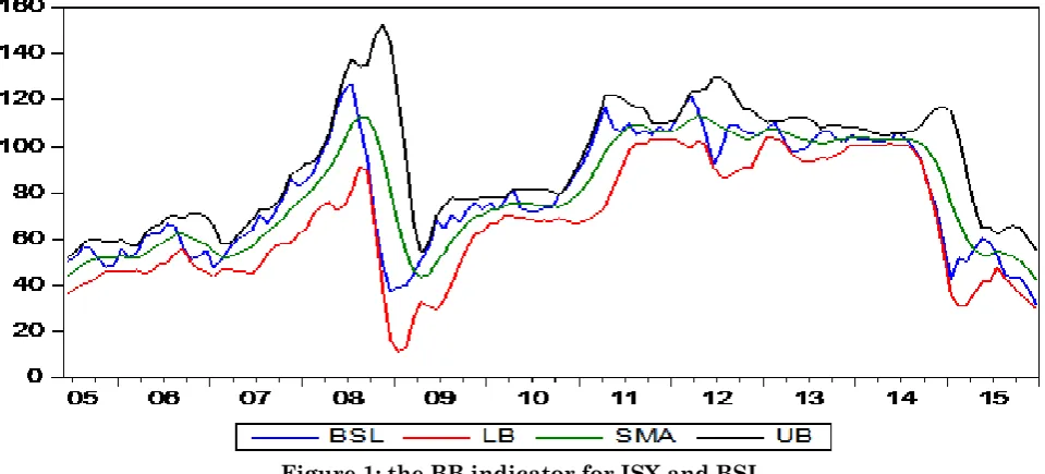
The study tried to employ the Bollinger
Bands-BB- (the results are reported in
appendix 3, and depicted in Figure 1) to analysis the volatility of the variables, the result can be summarized in the following points:
The analysis shows a relative
synchronization between the volatility of
BSL and ISX in different periods, it is very necessary to point out that the volatility in crude oil prices were more extreme compared to the volatility in the financial market, noting the relatively high volatility in 2005 in both markets.
The ISX witnessed a decline in volatility
during 2012 - 2013, in contrast, while BSL faced a high volatility level especially in 2012, continued to the subsequent years.
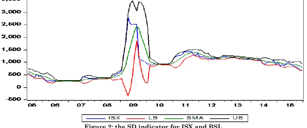
Figure 2: the SD indicator for ISX and BSL Standard Deviation Results
The standard deviation (the results are reported in appendix 4, and depicted in Figure 2)
shows that the BSL volatility is more severe compared to the ISX, despite the low volatility of BSL, but it was characterized by sharpness and continuity from the beginning of the time series until 2008, after that year, the volatility level was the highest, but the response of the financial market came after four months later.
After 2014, the BSL and ISX witnessed high synchronization volatility, reflecting the
deterioration of crude oil prices during that period and continued to fluctuate continuously until the end of the time series.
Source: Researcher’s calculation based on the data in App. 2 and calculated values in App.3
Correlation Results
Correlation Results between ISX and Oil Market Indicators
The analysis of the correlation between the
ISX index and the oil market indicators reveals a positive correlation during the study period. However, it is correlation with BSL higher than its correlation with Brent and West Texas. The correlation coefficients were 28%, 22.8% and 11.4%, respectively as shown in the table:
Table 1 shows the values of the ISX and oil
prices, as the positive correlation became very clear between ISX and BSL
especially after 2009, reflecting the ISX response to the volatility of crude oil prices.
In the most years, the growth of the
financial market was moving along with BSL direction, a positively or negatively, unlike the earliest years of the study, which showed a negative correlation between the markets, it might be acceptable considering to the short duration of trading in the market, the low confidence of investors in financial institutions in the country, the security and political instability, that contributed to reduce the correlation between crude oil prices and the performance of the financial market.
Table 1: the annual growth and correlations for ISX and BSL
Date ISX&BSL ISX&BRENT ISX&WTI
2005 (0.79146) (0.82878) (0.8439)
2006 (0.24282) (0.18417) (0.12149)
2007 0.640307 0.59072 0.644864
2008 (0.73523) (0.74634) (0.73137)
2009 0.014433 (0.05045) (0.04022)
2010 0.77973 0.748257 0.731278
2011 0.41227 0.439507 (0.19451)
2012 0.424457 0.392028 0.184939
2013 0.102767 0.076085 (0.45481)
2014 0.370804 0.404723 0.326957
2015 0.721728 0.71893 0.75466
Total Corr. 0.281319 0.228918 0.114277
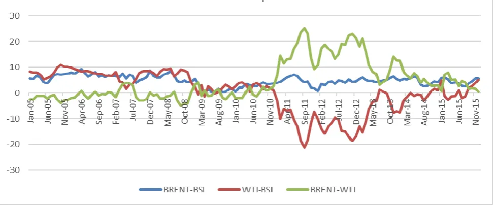
Figure 2: The oil benchmarks difference compared to BSL
Date BSL Annual G. ISX Index Annual G.
2005 27.39 -28.60
2006 -0.64 -33.81
2007 73.82 33.55
2008 -56.26 71.55
2009 85.03 51.28
2010 16.31 7.47
2011 14.87 16.82
2012 -4.69 2.76
2013 -2.22 -7.75
2014 -43.58 -18.27
2015 -24.65 -26.82
Source: Researcher’s calculation based on the data in App. 2
Correlation Results between BSL, Brent, and WTI
BSL is correlated with Brent more than its
correlation WTI. The correlation
coefficients were 99% and 95%,
respectively. At the same time, BSL correlation with Brent shows a stable pattern with 5$ average difference, the highest difference reached $ 9 in Apr2006, Dec2007 and Jun2008, which tended to
decline during the prices collapse in 2008 with a minimum difference $ 5, it can be pointed out that BSL was never traded at a lower level of Brent crude During that period, in contrast to its relationship with WTI, which fell below the BSL during 2011-2015.
BSL was the most volatile crude compared
Source: Researcher’s calculation based on the data in App. 2
Empirical Results
Unit Root testsTable (3) shows the unit test results of the variables at level according to the ADF & PP tests, at (5% -1%) significant level, the calculated value of the T statistic is less than
the critical value for the variables in both tests, which led to take the first difference in order to remove the spurious regression. The purpose was achieved, and then we decided to reject the null hypothesis and accept the alternative hypothesis, which means that all variables are integrated at level I (1).
Table 3: Unit Root Test
Unit Root Test as Level
PP Test ADF Test Variable
Prob. t-Stats Prob. t-Stats
0.1189 -2.88358 0.2718 -2.88358 α ISX
0.2382 -3.44449 0.1065 -3.44503 £α
0.2732 -2.88358 0.1667 -2.88375 α BSL
0.834 -3.44449 0.6236 -3.44476 £α
Unit Root Test at First Difference
PP Test ADF Test Variable
Prob. t-Stats Prob. t-Stats
0 -2.88375 0 -2.88375 α ISX
0 -3.44476 0 -3.44476 £α
0 -2.88375 0 -2.88375 α BSL
0 -3.44476 0 -3.44476 £α
Source: Researcher’s calculation based on the data in App. 2 and E views 9 Optimal Lag Selection
Table 4: Optimal lag selection
Lag LogL LR FPE AIC SC HQ
0 -1743.057 NA 8421162. 27.29777 27.38689* 27.33398* 1 -1718.476 47.24110 7365682.* 27.16369* 27.60932 27.34475 2 -1706.520 22.23066 7852171. 27.22688 28.02901 27.55279 3 -1690.095 29.51427* 7814848. 27.22023 28.37887 27.69099 4 -1679.571 18.25221 8542847. 27.30580 28.82094 27.92141 Source: Researcher’s calculation based on the data in App. 2 and Eviews 9
Before running the Johansson & Juselius
test, the determination of the optimal lag is required as a precondition to run the model. The results are reported in table (4) shows
that one-time lag satisfies the optimal time lag condition.
Table (5) summarizes the results of the Johansson & Juselius Cointegration test. As shown, the values of the Trace statistic are greater than the critical values at a 5% significant level with one vector, thus we can
reject the null hypothesis and accept the alternative hypothesis which indicated that there is a Co integration relationship between the variables, the decision confirmed tests, the Max and Trace tests.
Table 5: Johansson & Juselius test
Probability Value Alternative Hypothesis Null Hypothesis Critical Value Test Value J&J for ISX and BSL
0.1268 r = 1 r = 0 15.49471 12.68681
Trace Test
0.0339 r = 2 r ≥ 1 3.841466 4.497805
0.3598 r = 1 r = 0 8.189009 8.189009
Max Test
0.0339 r = 2 r ≥ 1 4.497805 4.497805
Probability Value Alternative Hypothesis Null Hypothesis Critical Value Test Value J&J for ISX and BRENT
0.1384 r = 1 r = 0 15.49471 12.40821
Trace Test
0.0339 r = 2 r ≥ 1 3.841466 4.500204
0.3881 r = 1 r = 0 14.26460 7.908008
Max Test
0.0339 r = 2 r ≥ 1 3.841466 4.500204
Probability Value Alternative Hypothesis Null Hypothesis Critical Value Test Value J&J for ISX and WTI
0.0830 r = 1 r = 0 15.49471 13.99905
Trace Test
0.0175 r = 2 r ≥ 1 3.841466 5.641442
0.3435 r = 1 r = 0 14.26460 8.357610
Max Test
0.0175 r = 2 r ≥ 1 3.841466 5.641442
Results of Granger Causality Test
The results of the test presented in Table (6), revealed the existence of three causality relationships in one direction, derived from the oil market variables (WTI, BRENT, BSL),
to the ISX by taking five time lags, considering the given time frame used in the study, the volatility of crude oil prices will be reflected on the financial market after five
months.
Table 6: Granger causality test
NO Causality Direction F - Ststs. Probability V.
BRENT → ISX 3.52835 0.0093
2 ISX → BRENT 0.27978 0.8906
3 BSL → ISX 3.52831 0.0093
4 ISX → BSL 0.25951 0.9033
5 WTI → ISX 4.51831 0.002
6 ISX → WTI 0.1696 0.9535
Source: Researcher’s calculation based on the data in App. 2 and E views 9
VECM Error Test Results
The results of the VECM model showed in appendix 1 indicated that there is a long-term equilibrium relationship arising from crude oil price indices (Basra, Brent and WTI crude) to the ISX index.
The results can be justified by the dependence of the Iraqi economy on the price of crude oil to finance the overall economic activity, then the oil prices volatility will have an important role in deriving the volatility of the financial market, in addition the macroeconomic trends. The results of VECM revealed that there is no long-term relationship between the ISX index and the
three oil market indices; this is a reasonable results considering the following reasons.
The weakness of the industrial sector in
Iraq, and the dominance of the banking sector on the financial market.
Low investment awareness among the
society.
The inefficiency of the market, as well as
the lack of integration of the Iraqi stock exchange with international markets due to lack usage of technology.
The limited financial instruments traded in
by non-economic factors, such as the political situation and the security chaos. The previous factors have constrained the role of the financial market in the economy, making it incapable of causing fluctuations of oil prices, and even restricted in receiving external price shocks.
Analyzing the Short Term Results of VECM
BSL time lag: The results of the VECM
model revealed a shift in the direction of the relationship between the BSL and the volatility of ISX. The results of appendix 1 show that the variables were negatively associated at the beginning of the period, then shifted to a positive relationship until the end of the time series, the results of the correlation analysis showed a variation in the correlation between the two variables, as the positive correlation increased after 2009 with a rising pattern.
Brent and WTI: They appear to be positively
correlated with ISX, any increase in oil benchmark prices in the current period, leads to a rise of 1.12% (Appendix 1) in the Iraqi stock market index in the coming period. This result indicates that the Iraqi economy has responded significantly to external shocks, especially the oil sector represents an external influencer.
Conclusions and Recommendations
Conclusions
There are three causal relationships in one
direction, derived from the oil market variables (WTI, BRENT, BSL), to the ISX, by taking five time lags.
arising from crude oil price indices (Basra, Brent and WTI crude) to the ISX index, while there was no influence from ISX to crude oil indicators.
The results of the VECM model revealed a
shift in the direction of the relationship between the BSL and the volatility of ISX. The results of appendix 1 show that the variables were negatively associated at the beginning of the period, then shifted to a positive relationship until the end of the time series.
There is a positive correlation between the
volatility of ISX index and the oil prices during the study period.
The ISX correlation with BSL was higher
than its correlation with Brent and WTI.
BSL is more strongly associated with Brent
than its relationship with WTI,
characterized by a stable pattern during the study period.
Recommendations
Diversifying the productive base of the
Iraqi economy to reduce the reliance of the economy on the oil sector, which will lead to reduce the effect of the oil prices on financial market?
Expanding the role of shareholding
companies as a modern model for the private sector, which increases the number of companies registered in the Stock market.
Adopting advanced electronic trading
systems to raise the efficiency of the financial market and make it more capable of reversing the market fundamentals [12-14].
References
1. Jung Wook Park, Ronald A, Rattia (2007)Oil price shocks and Stock markets in the U.S. and 13 European Countries. Columbia: University of Missouri-Columbia, MO 65211, U.S.A. 2. Samuel Imarhiagbe (2010) Impact of oil prices
on stock markets: Empirical evidence from selected major oil producing and consuming countries . Global Journal of Finance and Banking Issues 4( 4):15-31.
3. Fouquau Julien, Mohamed Arouri (2009) On the shortterm influence of oil price changes on stock markets in GCC countries: linear and nonlinear analyses. Economics Bulletin: Volume 29-2.
4. Sanjay Peters, Rumi Masih Lurion, De Mello (2011) Oil price volatility and stock price fluctuations in an emerging market: Evidence from South Korea. Energy Economics: 33: 975-986.
5. Tarak Nath Sahu, Debasish Mondal (2014) Crude Oil Price, Exchange Rate and Emerging Stock Market: Evidence from India. Jurnal Pengurusan. 42:75-87.
6. Iraq Stock Exchange website: http://www.isx-iq.net/isxportal/portal/sectorsDetails.html 7. US Energy Information Administration (2016)
8. Ahmad A, Al-Majali, Ghazi I Al-Assaf (2014) (edition 10-10). Long Run and Short run relationship between stock market index and main macroeconomic variables performance in Jordan . European Scientific Journal ،156-171. 9. Ayhan Kapusuzoglu (2011) (1). Relationships
between Oil Price and Stock Market: An Empirical Analysis from Istanbul Stock Exchange (ISE). International Journal of Economics and Finance: 3(6:(99-106.
10. Annette Brose Olsen (2014 ) Oil Price Shocks and Stock Market Returns: A study on Portugal, Ireland, Italy, Greece and Spain . Sweden: Master Thesis - Lund University – school of economics and management .
11. JMurphy J (1999) Technical Analysis of the Financial Markets. New York: New York Institiute of Finance.
12. Iraq Stock Exchange (2013).The annual Report of Iraq Stock Exchange. Baghdad: Iraq Stock Exchange.
13. The website of the Organization of Arab Petroleum Exporting Countries (OAPEC): http://oapecdbsys.oapecorg.org:8080/apex/f?p=1 01:8:0
14. Website of Federal Reserve Bank of St. Luis: https://fred.stlouisfed.org/series/POILWTIUSD M
Appendix -1: VECM Results
Source: Researcher’s calculation based on the data in App. 2 and Eviews 9
D(WTI) D(BRENT) D(BSL) D(ISX) Error Correction: -0.002797 -0.004885 -0.002968 -0.055592
Error correction term (0.03840) (0.00121) (0.00126) (0.00129) [-2.17414] [-3.88878] [-2.44718] [-1.44767] 0.0316 0.0002 0.0158 0.1502 Probability 0.000177 0.000941 -0.000125 -0.468846
D(ISX(-1)) (0.07854) (0.00248) (0.00257) (0.00263)
[ 0.06731] [ 0.36617] [-0.05057] [-5.96955] -1.203038 -1.982786 -1.939770 -6.213259
D(BSL(-1)) (16.3023) (0.51486) (0.53330) (0.54612)
[-2.20287] [-3.71797] [-3.76759] [-0.38113] 1.266696 1.773388 1.642179 1.122175 D(BRENT(-1)) (0.56331) (0.55008) (0.53106) (16.8154) [ 2.24866] [ 3.22386] [ 3.09226] [ 0.06673] -0.396679 -0.048503 0.024338 4.578621
D(WTI(-1)) (5.94465) (0.18774) (0.19447) (0.19914)
[-1.99192] [-0.24942] [ 0.12964] [ 0.77021] -0.069421 -0.084859 -0.086000 -0.876285
C (17.4974) (0.55260) (0.57239) (0.58616)
[-0.11843] [-0.14825] [-0.15563] [-0.05008] 0.153445 0.189732 0.160697 0.284704 R-squared 4.495207 5.807151 4.748338 7.870969 F-Statistic 0.000846 0.000075 0.000528 0.0000000
critical value for (F) at 5%
Appendix 2: The Used Data of the Study
Date BSL ISX Date BSL ISX Date BSL ISX
Jan-05 38.579 639.2 Jan-08 85.21 340.2 Jan-11 92.33 1164.4
Feb-05 40.014 726.1 Feb-08 88.8 361 Feb-11 99.52 1236.7
Mar-05 46.213 672 Mar-08 97.19 375.1 Mar-11 109.16 1269.8
Apr-05 45.738 563.7 Apr-08 103.28 373 Apr-11 117.05 1282.9
May-05 44.569 603.3 May-08 116.35 383.5 May-11 107.93 1316.7
Jun-05 50.591 566.3 Jun-08 124.46 381.5 Jun-11 106.65 1427.6
Jul-05 52.237 520.1 Jul-08 127 380.5 Jul-11 109.87 1424.5
Aug-05 57.097 451.3 Aug-08 109.16 389.8 Aug-11 105.07 1424.6
Sep-05 55.677 400.3 Sep-08 94.84 543.8 Sep-11 106.68 1451.8
Oct-05 51.392 532.5 Oct-08 67.99 471.2 Oct-11 105 1330.1
Nov-05 48.068 434 Nov-08 49.11 556.5 Nov-11 108.47 1273.2
Dec-05 49.147 456.4 Dec-08 37.27 583.6 Dec-11 106.06 1360.3
Jan-06 55.586 382.1 Jan-09 39.47 666.7 Jan-12 110.21 1216.6
Feb-06 52.324 293.9 Feb-09 39.66 1355.9 Feb-12 116.21 1223.6
Mar-06 54.008 254.5 Mar-09 44.94 1839.4 Mar-12 121.96 1223.3
Apr-06 61.175 284.2 Apr-09 51.18 2811.1 Apr-12 116.26 1180.6
May-06 62.321 258.1 May-09 56.47 2537.3 May-12 105.94 1155.3
Jun-06 62.38 255.8 Jun-09 68.18 2516.3 Jun-12 92.02 1160.5
Jul-06 66.489 254.2 Jul-09 64.32 2526.3 Jul-12 98.16 1142.2
Aug-06 65.419 260 Aug-09 70.73 2536.3 Aug-12 108.68 1178.1
Sep-06 56.4 269.2 Sep-09 67.3 1138.4 Sep-12 109.39 1174.9
Oct-06 51.532 271.1 Oct-09 72.63 1090.8 Oct-12 106.66 1191.2
Nov-06 52.314 259.5 Nov-09 75.55 1062.5 Nov-12 105.45 1250.6
Dec-06 55.229 252.9 Dec-09 73.03 1008.6 Dec-12 105.04 1250.2
Jan-07 47.63 259 Jan-10 75.74 939.6 Jan-13 107.51 1226.5
Feb-07 51.19 262.9 Feb-10 72.25 929.9 Feb-13 110.48 1232.7
Mar-07 55.99 287.5 Mar-10 77.17 907.1 Mar-13 104.17 1195.7
Apr-07 59.74 266 Apr-10 81.35 940.7 Apr-13 98.22 1204.8
May-07 61.79 249.7 May-10 73.15 927.4 May-13 98.23 1217.8
Jun-07 64.09 258.8 Jun-10 72.09 935.6 Jun-13 98.94 1170.5
Jul-07 70.53 409.5 Jul-10 72.14 927.5 Jul-13 103.24 1164.4
Aug-07 66.83 419 Aug-10 73.39 914.7 Aug-13 106.07 1185.7
Sep-07 72.14 385.5 Sep-10 73.7 905.5 Sep-13 106.61 1138.9
Oct-07 77.47 369.9 Oct-10 79.36 928.8 Oct-13 103.69 1153.6
Nov-07 86.26 346.3 Nov-10 82.14 957.2 Nov-13 101.63 1142.8
Dec-07 82.79 345.9 Dec-10 88.09 1009.8 Dec-13 105.12 1131.5
Jan-14 102.7 1125.6 Sep-14 94.49 1002 May-15 60.4 967.37
Feb-14 103.38 1093.7 Oct-14 83.57 999.1 Jun-15 58.6 1000.5
Mar-14 102.1 1073.6 Nov-14 73.94 1079.3 Jul-15 53.1 903.4
Apr-14 102.11 1105.8 Dec-14 57.94 920 Aug-15 44.3 872.03
May-14 103.16 1108.8 Jan-15 42.6 998.3 Sep-15 43.4 844.9
Jun-14 105.8 954.8 Feb-15 51.8 874.32 Oct-15 43.5 781.56
Jul-14 103.83 936.6 Mar-15 50.5 900.9 Nov-15 38.7 718.64
Aug-14 99.2 1001.4 Apr-15 55.6 870.03 Dec-15 32.1 730.56
Sources
Iraq Stock Exchange website: http://www.isx-iq.net/isxportal/portal/sectorsDetails.html
The website of the Organization of Arab Petroleum Exporting Countries (OAPEC):
Appendix 3: BB Results
BSL ISX
Date SMA UB LB SD SMA UB LB SD
Jun-05 44.28 52.30 36.26 4.01 628.43 744.58 512.29 58.07
Jul-05 46.56 54.56 38.56 4.00 608.58 748.80 468.37 70.11
Aug-05 49.41 58.19 40.63 4.39 562.78 699.00 426.56 68.11
Sep-05 50.98 60.29 41.68 4.65 517.50 658.93 376.07 70.71
Oct-05 51.93 59.97 43.88 4.02 512.30 648.76 375.84 68.23
Nov-05 52.51 58.61 46.41 3.05 484.08 602.42 365.75 59.17
Dec-05 52.27 58.76 45.78 3.24 465.77 558.85 372.68 46.54
Jan-06 52.83 59.77 45.89 3.47 442.77 538.93 346.60 48.08
Feb-06 52.03 57.83 46.23 2.90 416.53 562.21 270.86 72.84
Mar-06 51.75 56.96 46.55 2.60 392.23 582.46 202.01 95.11
Apr-06 53.38 62.07 44.69 4.34 350.85 505.77 195.93 77.46
May-06 55.76 65.11 46.41 4.67 321.53 468.80 174.26 73.63
Jun-06 57.97 66.21 49.72 4.12 288.10 377.38 198.82 44.64
Jul-06 59.78 69.75 49.81 4.98 266.78 298.87 234.70 16.04
Aug-06 61.97 69.99 53.94 4.01 261.13 282.16 240.11 10.51
Sep-06 62.36 68.86 55.87 3.25 263.58 284.37 242.80 10.39
Oct-06 60.76 71.21 50.31 5.22 261.40 274.34 248.46 6.47
Nov-06 59.09 71.09 47.09 6.00 261.63 274.37 248.90 6.37
Dec-06 57.90 69.77 46.02 5.94 261.15 274.92 247.38 6.88
Jan-07 54.75 65.82 43.69 5.53 261.95 274.51 249.39 6.28
Feb-07 52.38 58.10 46.67 2.86 262.43 274.88 249.99 6.22
Mar-07 52.31 57.84 46.79 2.76 265.48 287.98 242.99 11.25
Apr-07 53.68 61.39 45.97 3.85 264.63 286.60 242.67 10.98
May-07 55.26 64.85 45.67 4.80 263.00 287.55 238.45 12.28
Jun-07 56.74 68.37 45.11 5.81 263.98 287.28 240.69 11.65
Jul-07 60.56 72.74 48.37 6.09 289.07 399.19 178.95 55.06
Aug-07 63.16 72.60 53.72 4.72 315.08 457.27 172.90 71.09
Sep-07 65.85 74.77 56.93 4.46 331.42 479.57 183.27 74.08
Oct-07 68.81 79.28 58.34 5.24 348.73 486.15 211.32 68.71
Nov-07 72.89 87.49 58.28 7.30 364.83 471.19 258.47 53.18
Dec-07 76.00 89.73 62.28 6.86 379.35 436.03 322.67 28.34
Jan-08 78.45 92.62 64.28 7.09 367.80 423.43 312.17 27.82
Feb-08 82.11 93.45 70.77 5.67 358.13 389.83 326.44 15.85
Mar-08 86.29 98.30 74.28 6.00 356.40 382.58 330.22 13.09
Apr-08 90.59 105.11 76.07 7.26 356.92 384.24 329.60 13.66
May-08 95.60 118.85 72.36 11.62 363.12 394.56 331.68 15.72 Jun-08 102.55 130.71 74.39 14.08 369.05 398.64 339.46 14.79 Jul-08 109.51 137.75 81.28 14.12 375.77 390.85 360.68 7.54
Aug-08 112.91 134.47 91.34 10.78 380.57 391.58 369.56 5.51 Sep-08 112.52 135.26 89.77 11.37 408.68 529.94 287.43 60.63 Oct-08 106.63 147.18 66.09 20.27 425.05 549.10 301.00 62.02 Nov-08 95.43 152.74 38.12 28.66 453.88 603.65 304.11 74.88
Dec-08 80.90 145.18 16.61 32.14 487.57 647.62 327.51 80.03 Jan-09 66.31 121.15 11.46 27.42 535.27 709.24 361.29 86.99
Feb-09 54.72 96.20 13.24 20.74 696.28 1297.46 95.11 300.59
Jun-09 49.98 70.27 29.70 10.14 1954.45 3464.20 444.70 754.88 Jul-09 54.13 74.28 33.97 10.08 2264.38 3268.18 1260.59 501.90 Aug-09 59.30 77.83 40.78 9.26 2461.12 3054.28 1867.95 296.58
Sep-09 63.03 76.91 49.15 6.94 2344.28 3442.44 1246.13 549.08 Oct-09 66.61 77.07 56.14 5.23 2057.57 3391.48 723.65 666.96 Nov-09 69.79 77.13 62.44 3.67 1811.77 3241.57 381.97 714.90 Dec-09 70.59 78.12 63.07 3.76 1560.48 2935.58 185.39 687.55 Jan-10 72.50 78.29 66.71 2.89 1296.03 2412.41 179.66 558.19
Feb-10 72.75 78.34 67.16 2.79 1028.30 1181.35 875.25 76.52
Mar-10 74.40 78.08 70.71 1.84 989.75 1128.28 851.22 69.27
Apr-10 75.85 81.79 69.90 2.97 964.73 1071.90 857.57 53.58
May-10 75.45 81.73 69.16 3.14 942.22 1005.57 878.86 31.68
Jun-10 75.29 81.85 68.73 3.28 930.05 952.69 907.41 11.32
Jul-10 74.69 81.62 67.76 3.47 928.03 949.01 907.06 10.49
Aug-10 74.88 81.60 68.17 3.36 925.50 948.53 902.47 11.52
Sep-10 74.30 80.72 67.89 3.21 925.23 949.13 901.33 11.95
Oct-10 73.97 78.94 69.00 2.48 923.25 943.36 903.14 10.06
Nov-10 75.47 83.20 67.74 3.86 928.22 960.82 895.62 16.30
Dec-10 78.14 89.53 66.74 5.70 940.58 1010.24 870.93 34.83
Jan-11 81.50 95.46 67.54 6.98 980.07 1158.67 801.47 89.30
Feb-11 85.86 102.93 68.78 8.54 1033.73 1281.60 785.87 123.93 Mar-11 91.77 112.15 71.39 10.19 1094.45 1364.41 824.49 134.98 Apr-11 98.05 122.15 73.94 12.05 1153.47 1407.10 899.83 126.82
May-11 102.35 122.44 82.26 10.04 1213.38 1418.45 1008.32 102.53 Jun-11 105.44 121.00 89.88 7.78 1283.02 1443.08 1122.96 80.03 Jul-11 108.36 118.68 98.05 5.16 1326.37 1474.92 1177.82 74.28 Aug-11 109.29 116.91 101.66 3.81 1357.68 1496.31 1219.06 69.31
Sep-11 108.88 116.75 101.00 3.94 1388.02 1515.66 1260.37 63.82 Oct-11 106.87 110.23 103.51 1.68 1395.88 1500.36 1291.40 52.24 Nov-11 106.96 110.45 103.46 1.75 1388.63 1517.32 1259.95 64.34 Dec-11 106.86 110.42 103.30 1.78 1377.42 1502.23 1252.60 62.41
Jan-12 106.92 110.67 103.16 1.88 1342.77 1505.68 1179.85 81.46 Feb-12 108.77 116.23 101.31 3.73 1309.27 1473.75 1144.79 82.24 Mar-12 111.32 123.27 99.37 5.97 1271.18 1383.59 1158.78 56.20 Apr-12 113.20 124.07 102.32 5.44 1246.27 1361.63 1130.90 57.68
May-12 112.77 124.51 101.03 5.87 1226.62 1356.22 1097.01 64.80 Jun-12 110.43 129.75 91.12 9.66 1193.32 1251.29 1135.34 28.99 Jul-12 108.43 129.81 87.04 10.69 1180.92 1245.16 1116.68 32.12 Aug-12 107.17 127.43 86.91 10.13 1173.33 1225.18 1121.49 25.92
Sep-12 105.08 120.90 89.25 7.91 1165.27 1192.92 1137.62 13.82 Oct-12 103.48 116.07 90.88 6.30 1167.03 1199.34 1134.73 16.15 Nov-12 103.39 115.92 90.86 6.27 1182.92 1250.73 1115.11 33.91 Dec-12 105.56 112.90 98.23 3.67 1197.87 1277.79 1117.95 39.96
Jan-13 107.12 110.29 103.95 1.58 1211.92 1275.78 1148.05 31.93 Feb-13 107.42 111.37 103.47 1.97 1221.02 1278.22 1163.81 28.60 Mar-13 106.55 110.68 102.43 2.06 1224.48 1271.75 1177.22 23.63 Apr-13 105.15 112.59 97.70 3.72 1226.75 1268.38 1185.12 20.82
Jul-13 102.21 111.00 93.43 4.39 1197.65 1246.18 1149.12 24.26 Aug-13 101.48 107.75 95.20 3.14 1189.82 1227.04 1152.59 18.61 Sep-13 101.89 109.06 94.71 3.59 1180.35 1232.62 1128.08 26.14 Oct-13 102.80 109.22 96.37 3.21 1171.82 1222.01 1121.62 25.10
Nov-13 103.36 108.56 98.16 2.60 1159.32 1191.66 1126.97 16.17 Dec-13 104.39 107.83 100.96 1.72 1152.82 1189.01 1116.63 18.09 Jan-14 104.30 107.88 100.73 1.79 1146.35 1185.68 1107.02 19.66 Feb-14 103.86 107.09 100.62 1.62 1131.02 1168.73 1093.31 18.86 Mar-14 103.10 105.39 100.82 1.14 1120.13 1175.85 1064.41 27.86
Apr-14 102.84 105.16 100.52 1.16 1112.17 1159.51 1064.83 23.67 May-14 103.10 105.14 101.05 1.02 1106.50 1145.16 1067.84 19.33 Jun-14 103.21 105.72 100.70 1.25 1077.05 1190.85 963.25 56.90
Jul-14 103.40 105.89 100.90 1.25 1045.55 1188.94 902.16 71.70 Aug-14 102.70 106.70 98.70 2.00 1030.17 1169.34 891.00 69.58 Sep-14 101.43 108.80 94.06 3.68 1018.23 1152.66 883.81 67.21 Oct-14 98.34 113.46 83.23 7.56 1000.45 1109.71 891.19 54.63
Nov-14 93.47 116.17 70.78 11.35 995.53 1085.86 905.21 45.16 Dec-14 85.50 117.13 53.86 15.82 989.73 1093.28 886.19 51.77 Jan-15 75.29 115.13 35.45 19.92 1000.02 1092.02 908.01 46.00 Feb-15 67.39 103.78 31.00 18.19 978.84 1110.00 847.68 65.58
Mar-15 60.06 88.51 31.61 14.23 961.99 1102.55 821.42 70.28
Apr-15 55.40 74.56 36.23 9.58 940.48 1090.90 790.05 75.21
May-15 53.14 64.73 41.55 5.80 921.82 1016.00 827.64 47.09
Jun-15 53.25 65.04 41.46 5.89 935.24 1046.02 824.45 55.39
Jul-15 55.00 62.15 47.85 3.57 919.42 1015.84 823.00 48.21
Aug-15 53.75 64.44 43.06 5.35 919.04 1016.19 821.89 48.57
Sep-15 52.57 65.72 39.41 6.58 909.71 1021.66 797.75 55.98
Oct-15 50.55 64.88 36.22 7.17 894.96 1041.80 748.12 73.42
Nov-15 46.93 60.43 33.44 6.75 853.51 1032.16 674.85 89.33
Dec-15 42.52 55.17 29.87 6.32 808.52 948.14 668.89 69.81
Source: Researcher’s calculation based on the data in App. 2
Appendix 4 : SD Results
Date BSL ISX Date BSL ISX Date BSL ISX
Feb-05 0.72 43.45 May-08 6.54 5.25 Aug-11 2.40 0.05
Mar-05 3.10 27.05 Jun-08 4.06 1.00 Sep-11 0.81 13.60
Apr-05 0.24 54.15 Jul-08 1.27 0.50 Oct-11 0.84 60.85
May-05 0.58 19.80 Aug-08 8.92 4.65 Nov-11 1.74 28.45
Jun-05 3.01 18.50 Sep-08 7.16 77.00 Dec-11 1.21 43.55
Jul-05 0.82 23.10 Oct-08 13.43 36.30 Jan-12 2.08 71.85
Aug-05 2.43 34.40 Nov-08 9.44 42.65 Feb-12 3.00 3.50
Sep-05 0.71 25.50 Dec-08 5.92 13.55 Mar-12 2.88 0.15
Oct-05 2.14 66.10 Jan-09 1.10 41.55 Apr-12 2.85 21.35
Nov-05 1.66 49.25 Feb-09 0.09 344.60 May-12 5.16 12.65
Dec-05 0.54 11.20 Mar-09 2.64 241.75 Jun-12 6.96 2.60
Jan-06 3.22 37.15 Apr-09 3.12 485.85 Jul-12 3.07 9.15
Feb-06 1.63 44.10 May-09 2.65 136.90 Aug-12 5.26 17.95
Mar-06 0.84 19.70 Jun-09 5.86 10.50 Sep-12 0.35 1.60
Apr-06 3.58 14.85 Jul-09 1.93 5.00 Oct-12 1.37 8.15
May-06 0.57 13.05 Aug-09 3.21 5.00 Nov-12 0.60 29.70
Aug-06 0.54 2.90 Nov-09 1.46 14.15 Feb-13 1.49 3.10
Sep-06 4.51 4.60 Dec-09 1.26 26.95 Mar-13 3.16 18.50
Oct-06 2.43 0.95 Jan-10 1.36 34.50 Apr-13 2.98 4.55
Nov-06 0.39 5.80 Feb-10 1.75 4.85 May-13 0.01 6.50
Dec-06 1.46 3.30 Mar-10 2.46 11.40 Jun-13 0.35 23.65
Jan-07 3.80 3.05 Apr-10 2.09 16.80 Jul-13 2.15 3.05
Feb-07 1.78 1.95 May-10 4.10 6.65 Aug-13 1.42 10.65
Mar-07 2.40 12.30 Jun-10 0.53 4.10 Sep-13 0.27 23.40
Apr-07 1.88 10.75 Jul-10 0.02 4.05 Oct-13 1.46 7.35
May-07 1.03 8.15 Aug-10 0.63 6.40 Nov-13 1.03 5.40
Jun-07 1.15 4.55 Sep-10 0.16 4.60 Dec-13 1.75 5.65
Jul-07 3.22 75.35 Oct-10 2.83 11.65 Jan-14 1.21 2.95
Aug-07 1.85 4.75 Nov-10 1.39 14.20 Feb-14 0.34 15.95
Sep-07 2.66 16.75 Dec-10 2.98 26.30 Mar-14 0.64 10.05
Oct-07 2.67 7.80 Jan-11 2.12 77.30 Apr-14 0.01 16.10
Nov-07 4.40 11.80 Feb-11 3.60 36.15 May-14 0.52 1.50
Dec-07 1.74 0.20 Mar-11 4.82 16.55 Jun-14 1.32 77.00
Jan-08 1.21 2.85 Apr-11 3.95 6.55 Jul-14 0.98 9.10
Feb-08 1.80 10.40 May-11 4.56 16.90 Aug-14 2.32 32.40
Mar-08 4.20 7.05 Jun-11 0.64 55.45 Sep-14 2.36 0.30
Apr-08 3.05 1.05 Jul-11 1.61 1.55 Oct-14 5.46 1.45
Nov-14 4.82 40.10 Feb-15 4.60 61.99 May-15 2.40 48.67
Dec-14 8.00 79.65 Mar-15 0.65 13.29 Jun-15 0.90 16.57
Jan-15 7.67 39.15 Apr-15 2.55 15.44 Jul-15 2.75 48.55
Aug-15 4.40 15.69 Oct-15 0.05 31.67 Dec-15 3.30 5.96
Sep-15 0.45 13.57 Nov-15 2.40 31.46