C
2013. The American Astronomical Society. All rights reserved. Printed in the U.S.A.
A CANDELS–3D-HST SYNERGY: RESOLVED STAR FORMATION PATTERNS AT 0.7
< z <
1.5
Stijn Wuyts1, Natascha M. F ¨orster Schreiber1, Erica J. Nelson2, Pieter G. van Dokkum2, Gabe Brammer3, Yu-Yen Chang4, Sandra M. Faber5, Henry C. Ferguson6, Marijn Franx7, Mattia Fumagalli7, Reinhard Genzel1,
Norman A. Grogin6, Dale D. Kocevski8, Anton M. Koekemoer6, Britt Lundgren9, Dieter Lutz1, Elizabeth J. McGrath10, Ivelina Momcheva2, David Rosario1, Rosalind E. Skelton11, Linda J. Tacconi1,
Arjen van der Wel4, and Katherine E. Whitaker12
1Max-Planck-Institut f¨ur extraterrestrische Physik, Postfach 1312, Giessenbachstr., D-85741 Garching, Germany;[email protected] 2Astronomy Department, Yale University, New Haven, CT 06511, USA
3European Southern Observatory, Alonson de C´ordova 3107, Casilla 19001, Vitacura, Santiago, Chile 4Max-Planck-Institut f¨ur Astronomie, K¨onigstuhl 17, D-69117 Heidelberg, Germany
5UCO/Lick Observatory, Department of Astronomy and Astrophysics, University of California, Santa Cruz, CA 95064, USA 6Space Telescope Science Institute, 3700 San Martin Drive, Baltimore, MD 21218, USA
7Leiden Observatory, Leiden University, P.O. Box 9513, 2300 RA Leiden, The Netherlands 8Department of Physics and Astronomy, University of Kentucky, Lexington, KY 40506, USA
9Department of Astronomy, University of Wisconsin-Madison, Madison, WI 53706, USA 10Department of Physics and Astronomy, Colby College, Waterville, ME 0490, USA 11South African Astronomical Observatory, Observatory Road, 7925 Cape Town, South Africa
12Astrophysics Science Division, Goddard Space Flight Center, Greenbelt, MD 20771, USA
Received 2013 July 1; accepted 2013 October 18; published 2013 December 3
ABSTRACT
We analyze the resolved stellar populations of 473 massive star-forming galaxies at 0.7 < z < 1.5, with multi-wavelength broadband imaging from CANDELS and Hαsurface brightness profiles at the same kiloparsec resolution from 3D-HST. Together, this unique data set sheds light on how the assembled stellar mass is distributed within galaxies, and where new stars are being formed. We find the Hαmorphologies to resemble more closely those observed in the ACSIband than in the WFC3Hband, especially for the larger systems. We next derive a novel prescription for Hα dust corrections, which accounts for extra extinction toward Hii regions. The prescription leads to consistent star formation rate (SFR) estimates and reproduces the observed relation between the Hα/UV luminosity ratio and visual extinction, on both a pixel-by-pixel and a galaxy-integrated level. We find the surface density of star formation to correlate with the surface density of assembled stellar mass for spatially resolved regions within galaxies, akin to the so-called “main sequence of star formation” established on a galaxy-integrated level. Deviations from this relation toward lower equivalent widths are found in the inner regions of galaxies. Clumps and spiral features, on the other hand, are associated with enhanced Hαequivalent widths, bluer colors, and higher specific SFRs compared to the underlying disk. Their Hα/UV luminosity ratio is lower than that of the underlying disk, suggesting that the ACS clump selection preferentially picks up those regions of elevated star formation activity that are the least obscured by dust. Our analysis emphasizes that monochromatic studies of galaxy structure can be severely limited by mass-to-light ratio variations due to dust and spatially inhomogeneous star formation histories.
Key words: galaxies: high-redshift – galaxies: stellar content – galaxies: structure – stars: formation Online-only material:color figures
1. INTRODUCTION
Studies of galaxy evolution from the peak of cosmic star formation to the present day have matured tremendously over the past two decades. Initially, efforts focused on the detection and selection of distant blobs of light by means of color selec-tions (Steidel et al.1996; Franx et al.2003; Daddi et al.2004), of which generally brighter subsets were confirmed spectro-scopically. Gradually, galaxy-integrated photometry over ever increasing wavelength baselines, from the rest-frame UV to infrared (IR), enabled inferences of the global stellar popula-tion properties such as stellar mass, age, and star formapopula-tion rate (SFR; Papovich et al.2001; F¨orster Schreiber et al.2004; Shapley et al.2005). Alongside developments on the stellar pop-ulation front, deep-field observations carried out with theHubble Space Telescope(HST) have played a pivotal role in opening up the distant universe for resolved, morphological analyses (e.g., Williams et al.1996; Giavalisco et al. 2004; Rix et al. 2004;
Koekemoer et al.2007). Initially, such look-back surveys were predominantly monochromatic, or at most spanning a limited number of bands probing the rest-frame UV emission, which is dominated by young O and B stars.
set, several works have contrasted monochromatic structural measurements to galaxy-integrated stellar population properties (Wuyts et al. 2011b; Weinzirl et al. 2011; Szomoru et al.
2011; Bell et al. 2012; Wang et al. 2012; Kartaltepe et al.
2012; Bruce et al.2012). Overall, these authors found strong correlations between structure and stellar populations (i.e., a “Hubble sequence”) to be present out to at leastz ∼2.5 (see also Franx et al.2008; Kriek et al.2009a). Star-forming galaxies (SFGs) residing on the SFR–mass “main sequence” relation (Noeske et al.2007; Elbaz et al.2007,2011; Daddi et al.2007) tend to be the largest at their mass, and are best characterized by exponential disk profiles, while quiescent galaxies lying below the main sequence have higher S´ersic indices, i.e., are more bulge-dominated (Wuyts et al.2011b; although see Barro et al.
2013for interesting sub-populations deviating from this overall trend). This implies bulge growth and quenching are intimately connected.
The molecular gas content of normal SFGs is known to in-crease rapidly with look-back time, to gas mass fractions of
∼0.33 (0.47) at z ∼ 1.2 (2.2) (Tacconi et al. 2010, 2013; Daddi et al.2010). Simple stability arguments predict such gas-rich systems to be prone to gravitational collapse on scales of
∼1 kpc. Indeed, such features, and more generally irregular mor-phologies, have been abundantly reported in high-redshift SFGs (albeit on monochromatic, and often rest-UV or Hαimages; see, e.g., Elmegreen et al.2004,2009b; Genzel et al.2008,2011). Analytic work as well as hydrodynamic simulations have pro-posed that the giant clumps may migrate inward via dynamical friction and tidal torques, thereby providing an alternative chan-nel to bulge formation to the conventional merger scenario (e.g., Noguchi1999; Immeli et al.2004a,2004b; Bournaud et al.2007; Dekel et al.2009). In part, the efficiency of such violent disk instabilities in driving significant bulge growth is subject to the longevity of the clumps, which may be limited by vigorous out-flows driven by internal star formation (e.g., Newman et al.2012; Genel et al.2012; Hopkins et al.2012). However, several studies argued that even if the clumps do not remain bound, torques in unstable disks will still lead to an enhanced gas inflow rate with respect to stable configurations (Krumholz & Burkert 2010; Bournaud et al.2011; Genel et al.2012; Cacciato et al.2012).
Additional clues on the emergence of bulges and the role or nature of clumps can come from studies of the resolved stellar populations within galaxies. Here too, Advanced Camera for Surveys (ACS) + WFC3 imaging from CANDELS and pre-existing campaigns offer the capability to expand sensitively on pioneering work by, e.g., Abraham et al. (1999), Elmegreen et al. (2009a), and F¨orster Schreiber et al. (2011a, 2011b). Wuyts et al. (2012) carried out seven-band stellar population modeling on a (binned) pixel-by-pixel basis for 649 massive (logM∗ > 10) SFGs at 0.5 < z < 2.5, the largest and only mass-complete sample of SFGs subject to such a detailed analysis to date. Translating the internal variations in intensity and color to spatial distributions of more physically relevant quantities such as stellar mass, SFR, age, and extinction, these authors found high-redshift SFGs to be smoother and more compact in mass than in light, with color variations driven by a combination of radial extinction gradients and spatial (short-term) fluctuations in the star formation history (see also F¨orster Schreiber et al.2011a,2011b; Guo et al.2012; Lanyon-Foster et al.2012; Szomoru et al. 2013). In particular, Wuyts et al. (2012) and Guo et al. (2012) found regions with enhanced surface brightness with respect to the underlying disk to be characterized by enhanced levels of star formation and younger
ages than interclump regions at the same galactocentric distance. Typical inferred clump ages of 100–200 Myr atz∼2 imply that the clumps correspond to short-lived star-forming phenomena, possibly limited in lifetime by stellar feedback. If inward clump migration is taking place, this should happen efficiently on timescales similar to the orbital timescale. Radial age gradients of clumps (F¨orster Schreiber et al.2011b; Guo et al.2012) may signal such migrational processes to be at play. Atz∼1, which is the epoch we focus on in this paper, the physics leading to regions of excess surface brightness and locally enhanced star formation may be a mix of the above violent disk instabilities frequently studied atz ∼ 2 and more conventional processes known from nearby SFGs. That is, gas fractions can still be sufficiently high to cause gravitational collapse while timescales become long enough for other instabilities, such as spiral density waves, to arise (the latter are only in rare cases seen atz∼2; see Law et al.2012). We note, as we did in our previous work, that while for simplicity we occasionally use the same short-hand “clump” terminology as Wuyts et al. (2012), the specific diagnostic identifying enhanced surface brightness regions does not discriminate between round knots or spiral features.
Despite the richness of the HST broadband data sets, the multi-wavelength sampling available at high resolution is still modest in comparison to state-of-the-art spectral energy distri-butions (SEDs) on a galaxy-integrated level. The latter span up to 30+ medium and broad bands from 0.3 to 8μm (e.g., Ilbert et al. 2009; Whitaker et al. 2011; Spitler et al. 2012), com-plemented further by mid-IR-to-far-IR photometry, and probe dust-obscured star formation within at least the more massive SFGs (e.g., Magnelli et al. 2013). The performance and lim-itations of broadband SED modeling as a tool to infer stellar population properties have been abundantly tested on synthetic observations of simulated galaxies (Wuyts et al.2009; Lee et al.
2009; Pforr et al.2012; Mitchell et al. 2013). It is clear that, while four to sevenHSTbroad bands may be sufficient to re-construct stellar mass distributions,13some level of degeneracy (e.g., between age and dust extinction) will be inherent to the inferences made on a pixel-by-pixel basis when SEDs span the relatively narrow wavelength range from observedBtoHband. Additional empirical constraints would allow us to test and build on the more model-sensitive findings from Wuyts et al. (2012). The 3D-HST legacy program (van Dokkum et al. 2011; Brammer et al. 2012) and GOODS-North grism survey GO-11600 (PI: B. Weiner), together covering all five CANDELS fields, provide two such empirical constraints. First, the grism data yields spectroscopic redshifts for thousands of galaxies, eliminating an important source of uncertainty that propagates in all derived stellar population properties. Second, each dispersed galaxy image can be considered as a continuum with superposed resolved line emission maps atHSTresolution. After subtracting the continuum underlying the Hαemission ofz∼1 galaxies, we are therefore left with an independent SFR diagnostic probing the same kiloparsec scales as the CANDELS multi-wavelength broadband imaging. The additional information furthermore allows us to better constrain the effects of extinction. Nelson et al. (2012,2013) demonstrated the power of this technique by contrasting the stacked one-dimensional HαandH-band surface brightness profiles. They found the extent of the ionized gas and
stellar light profiles to be similar for small galaxies. The ionized gas component of the larger galaxies, on the other hand, exhibit larger scale lengths than the stellar component, consistent with an inside-out growth scenario. As is the case for rest-optical light profiles, the Hαemission of SFGs in their sample is best characterized by an exponential disk profile.
In this paper, we build on the analyses by Nelson et al. (2012, 2013) and Wuyts et al. (2012) by combining the re-solved Hαinformation onz∼1 SFGs with pixel-by-pixel stel-lar population modeling of their multi-wavelength broadband photometry. The present work has strong connections to a very comprehensive exploration of Hαand SFR profiles throughout the two-dimensional (2D) SFR–mass space (E. Nelson et al. in preparation). While restricting the analysis to systems with well-detected line emission, we expand the sample with respect to previous work by exploiting the data in all five CANDELS/ 3D-HST fields (see the sample description in Section2). We discuss the methodology to derive stellar population properties such as star formation and surface mass density in Section3. Here, we place a special emphasis on dust corrections, and in particular extra extinction toward the Hiiregions from which the Hαline emission originates, using UV+IR based SFRs as an additional calibrator. After a visual impression of characteristic features in the Hαand broadband images (Section4), we quan-tify the correspondence between Hαand broadband morpholo-gies at different wavelengths (Section5.1), compare emission line diagnostics to stellar population properties derived from broadband information alone (Section5.2), and finally contrast the Hαand corresponding star formation properties of galaxy centers, clumps/spiral arms, and underlying disks within our sample of SFGs with logM∗ >10 (Section5.3).
Throughout this paper, we quote magnitudes in the AB sys-tem, assume a Chabrier (2003) initial mass function (IMF) and adopt the following cosmological parameters: (ΩM,ΩΛ, h) =
(0.3,0.7,0.7).
2. OBSERVATIONS AND SAMPLE
HSTbroadband imaging from CANDELS and pre-existing surveys, together withHSTgrism spectroscopy from 3D-HST, form the core data set on which this paper is based. In addition, our sample definition makes use of the wealth of ancillary data collected in the five CANDELS/3D-HST fields, including multiple medium-band and broadband imaging campaigns from the ground, and space-based photometry fromSpitzer/IRAC, Spitzer/MIPS, and Herschel/PACS. We derived the galaxy-integrated stellar masses and SFRs based thereupon following identical procedures to Wuyts et al. (2011b). That is, the SFRs that enter the sample selection criteria are based on a ladder of SFR indicators, using UV+PACS for PACS-detected galaxies and UV+MIPS 24μm for MIPS-detected galaxies; SFRs from SED modeling (which also yield the stellar masses) are used for sources without IR detection. The 3D-HST catalogs with consistent multi-wavelength photometry that serve as input to the galaxy-integrated SED modeling are presented by R. Skelton et al. (in preparation).
2.1. CANDELS HST Imaging
CANDELS provides deep WFC3 imaging of five disjoint fields on the sky: GOODS-South, GOODS-North, COSMOS, UDS, and EGS, totaling approximately 800 arcmin2. Point-source limiting depths vary fromH=27.0 mag in CANDELS/ Wide toH=27.7 mag in CANDELS/Deep (the central halves
of the GOODS fields). We refer the reader to Grogin et al. (2011) for an overview of the survey layout and Koekemoer et al. (2011) for details on the data reduction. Other HST imaging that enters our analysis includes the GOODS ACS campaigns (Giavalisco et al.2004) and subsequent ACS epochs taken as part of the HSTsupernovae search, COSMOS/ACS (Koekemoer et al.2007), AEGIS/ACS (Davis et al.2007), and ERS/WFC3 (PI: O’Connell) observations. Together, these yield B435V606i775z850J125H160 photometry in the GOODS fields, with an additionalY098coverage of the ERS region (top third
of GOODS-South), and Y105 coverage of the CANDELS/
Deep regions. For the remaining fields, SEDs are sampled by V606I814J125H160photometry.
2.2. 3D-HST Grism Spectroscopy
Brammer et al. (2012) describe in detail the specifications of the 3D-HST legacy program. Briefly, 3D-HST14 covers three quarters (625 arcmin2) of the CANDELS treasury survey area, and naturally our sample will be drawn from the region where the two data sets overlap. In this paper, we make use of the two orbit depth WFC3/G141 grism exposures, but note that in parallel two to four orbits of ACS/G800L grism data were taken as part of the program. The WFC3/G141 grism data reach a 5σ emission-line sensitivity of∼5×10⁻¹⁷erg s−1cm−2and
cover a wavelength range from 1.1 to 1.6 μm. We make use of the v2.1 internal release by the 3D-HST team, which differs most significantly from the data handling described by Brammer et al. (2012) in that the half-pixel dithered exposures are combined by interlacing rather than drizzling, thereby reducing the correlated noise. The extraction of grism spectra followed the steps outlined by Brammer et al. (2012). As part of the extraction pipeline, a spectral model is constructed that, once convolved with the F140W pre-image of the galaxy that serves as a template, best fits the observed grism spectrum. In this process, neighbors are treated simultaneously to reduce contamination effects. Redshifts are fitted to the combination of available broadband and grism information. In practice, for the sample of line-emitting galaxies analyzed in this paper, the ancillary broadband data only serves in the redshift determination to prevent line misidentifications.
2.3. Sample Definition
The adopted redshift range of 0.7< z <1.5 for our sample is dictated by the requirement that the Hαemission falls within the WFC3/G141 wavelength coverage. We next apply the same basic criteria to select massive SFGs as Wuyts et al. (2012), namely logM∗ > 10 and a specific SFR (SSFR)> 1/tHubble.
The depth of the H-band selected parent catalogs guarantees completeness down to this mass limit (and in fact more than an order of magnitude below). Over the entire CANDELS/3D-HST area with coverage by the G141 grism spectroscopy and at least fourHSTbroad bands, this amounts to 1844 massivez∼1 SFGs.
Subsequent selection criteria serve to optimize the quality of our inferences on resolved Hαproperties at the expense of compromising the mass completeness of our SFG sample. For our final sample, we require galaxies to have secure redshifts with well-covered Hαemission detected at the 8σ significance level. We furthermore apply a conservative screening against
Table 1
Sample Selection of Massive SFGs at 0.7< z <1.5 with HαMaps from 3D-HST
Selection N(Total) N(GOODS-S) N(GOODS-N) N(EGS) N(UDS) N(COSMOS)
0.7< z <1.5 & logM∗>10 3115 609 656 340 692 818
. . .& SSFR>1/tHubble 1844 359 381 206 433 465
. . .& HαS/N>8 636 109 176 96 130 125
. . .& no contamination or continuum residuals 506 95 143 72 110 86
. . .& Final samplea 473 85 129 69 108 82
Note.aCompact or heavily point-source-dominated sources with an X-ray counterpart are excluded from the final sample.
objects whose grism spectra are contaminated by neighboring sources, as identified based on products of the 3D-HST pipeline, supplemented with a visual inspection. In this step, we also weed out a small number of sources with prominent residuals over the full wavelength range after subtraction of the continuum model produced by the 3D-HST extraction and fitting pipeline. Finally, we exclude 33 bright X-ray detected objects for which the compact nature of their HST imaging could hint at a significant non-stellar contribution to both the broadband and the Hαline emission. Before the latter cut, the overall fraction of X-ray detected sources in the Hαsample exceeds the respective X-ray detected fraction determined for the complete parent sample of massive SFGs by a factor of 1.5 (∼12% versus
∼8%15). A possible explanation for this difference may be a tendency for actively star-forming, line-emitting galaxies to more frequently host active galactic nucleus (AGN) activity (e.g., Santini et al.2012; Trump et al.2013). In addition, since the Hαand [Nii] emission lines are blended in the WFC3 grism data (see Section3.2), the enhanced [Nii]/Hαratios of AGN-hosting galaxies may push more of them over the signal-to-noise threshold for line emission. In our final sample, the only X-ray detected sources remaining are located in GOODS-South (16) and GOODS-North (7). We note that in these deep X-ray fields (4 Ms and 2 Ms exposure, respectively), not all X-ray detected sources are necessarily AGNs. Moreover, no evidence for point source contamination is seen in theirHSTimaging. We break down our final sample and the intermediate selection steps by field in Table1.
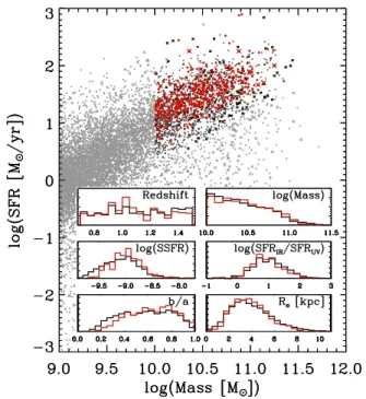
It is important to note that our final sample of 473 massive SFGs spans the entire range in mass and SFR of typical main-sequence galaxies above log(M∗)=10 (see Figure1). The inset panels in Figure1present a closer look at the relation between the Hαsample and the underlying complete parent population of massive SFGs at 0.7< z <1.5. At first glance, the samples are well matched in redshift, mass, star formation activity, obscuration (SFRIR/SFRUV), axial ratio, and size, in terms of
dynamic range spanned as well as the distribution within that range. In more detail, the Hαsample shows subtle biases against the lowest SSFR systems, against the most obscured galaxies at a given SFR, and, related, against the most edge-on galaxies. The similarity between the two samples is encouraging, as it implies that the analysis of the Hα sample presented in this paper can reveal generic insights for the entire massive SFG population during the transition from the peak of cosmic star formation to the initial phases of its decline.
15 The percentages quoted are for the sum of all five CANDELS/3D-HST fields. While the absolute percentages are field-dependent due to varying depth of the X-ray imaging, the relative factor of 1.5 between the Hαand parent sample is similar for all fields.
Figure 1.Location of our massive SFG sample (red) in SFR–mass space, overplotted on the distribution of the overall galaxy population at 0.7< z <1.5. Crosses mark X-ray-detected sources. Inset panels show the distribution in redshift, stellar mass ([M]), specific SFR ([yr−1]), and obscuration level (SFRIR/SFRUV) for the Hαsample analyzed in this paper (red) compared to the complete sample of SFGs above logM∗=10 (black).
(A color version of this figure is available in the online journal.)
3. METHODOLOGY
3.1. Modeling of the Broadband SEDs
The three basic steps toward resolved SED modeling are point-spread function (PSF) matching, pixel binning, and stellar population synthesis modeling of the individual spatial bins. Each of these steps is described in depth by Wuyts et al. (2012). Briefly, we work at the WFC3H160resolution of 0.18 and used
the Iraf PSFMATCH algorithm to build kernels to bring all shorter wavelength images to the same PSF width and shape. We next applied the Voronoi binning scheme by Cappellari & Copin (2003) to group neighboring pixels together in bins so as to achieve a minimum signal-to-noise level of 10 per bin. We applied the Voronoi binning scheme to the WFC3H160maps.
to Wuyts et al. (2011b,2012). Since all galaxies in our sample have spectroscopically confirmed redshifts from the Hα line detection in the grism data (and in half of the cases confirmed independently by ground-based spectroscopic campaigns), we fix the redshift to its spectroscopically determined value in our SED fitting, hence reducing the number of free parameters by one. In addition, we assume the stars have a fixed, solar metallicity. While this assumption is frequently adopted in the literature on stellar populations of massivez∼1 galaxies, we caution that additional constraints and further investigations are needed to address the validity and impact of this assumption for resolved studies on kiloparsec scales. We follow Salim et al. (2007) in adopting parameter values marginalized over the multi-dimensional grid explored in SED fitting, as this approach proved most robust (compared to, e.g., adopting the least squares solution) in the limit of poorly sampled SEDs. Additional notes on the reliability of the broadband SED modeling and its impact on the results presented in this paper are discussed in the
Appendix.
3.2. Extracting HαEmission Line Maps
In order to extract Hαemission line maps, we follow Nelson et al. (2012, 2013), and subtract the continuum model from the observed 2D grism spectrum. The resulting residual image is then mapped to the CANDELS frame using redshift and astrometric information, and contains the emission line surface brightness distribution without imposed prior on its morphology. At the spectral resolution ofδv ≈1000 km s−1, Hαand [Nii]
λλ6548+6583 are blended. As we lack additional constraints, we apply throughout the paper a simple downscaling of the observed emission line flux by a factor of 1.2, and refer to this quantity as the Hα flux. In reality, [Nii]/Hα ratios may vary between galaxies as well as spatially within galaxies (see, e.g., Liu et al. 2008; Yuan et al. 2012, 2013; Queyrel et al.
2012; Swinbank et al.2012; Jones et al. 2013; N. M. F¨orster Schreiber et al. in preparation). However, restricting the above spectroscopic samples to the same redshift range as adopted in this paper, the scatter in [Nii]/Hαis substantial compared to any systematic trend, if present, with galaxy mass above log(M∗) =10. Furthermore, the [Nii]/Hα gradients reported based on adaptive optics assisted observations are typically shallow (N. M. F¨orster Schreiber et al. in preparation). We conclude that a higher order correction than the uniform scaling factor we apply is not justified by the present data.
Again following Nelson et al. (2013), we apply a wedge-shaped mask to regions that could potentially be affected by [Sii]λλ6716+6731 line emission (redward from Hαalong the dispersion axis), which can mimic the appearance of an off-center clump in the Hαmaps.
3.3. Dust Corrections to the HαEmission
3.3.1. Birth Clouds and Diffuse Interstellar Dust
Proper extinction corrections are critical for the physical interpretation of dust-sensitive SFR tracers. This applies to short wavelength (rest-UV) broadband indicators, motivating to a large extent programs such as CANDELS. While at the longer, rest-optical wavelengths, attenuation laws predict a significantly suppressed impact by dust; this may not be the case for the Hα emission at 6563 Å, depending on the geometry of dust and stars. Hα emission originates from Hii regions immediately surrounding young star-forming regions, which are known to be often associated with enhanced levels of obscuring material.
As such, the nebular emission emerging near massive O stars that have not yet dispersed or escaped from their dust-rich birth clouds will be subject to extra extinction with respect to continuum light at the same wavelength that is produced by the bulk of the stars (no longer embedded in the molecular clouds in which they once formed). The observed (i.e., attenuated) Hα flux then relates to the intrinsic fluxFHα,intas
FHα,obs=FHα,int10−0.4Acont10−0.4Aextra, (1)
where Acont represents the attenuation by diffuse dust in the
galaxy andAextra represents the attenuation happening locally
in the birth cloud. The latter have a negligible covering factor and therefore affect no other galaxy light than that emerging from the respective star-forming region itself. The geometrical picture sketched here relates intimately to the framework of the Charlot & Fall (2000) model and subsequent refinements by, e.g., Wild et al. (2011), Pacifici et al. (2012), and Chevallard et al. (2013).
Empirical evidence for the need of an extra extinction correction to Hα(i.e.,Aextra=0) was first presented for a sample
of nearby starburst galaxies by Calzetti et al. (1994,2000). Also at larger look-back times, evidence for differential extinction between nebular regions and the bulk of the stars has been mounting, from arguments based on the observed Hαequivalent widths (EWs; van Dokkum et al.2004; F¨orster Schreiber et al.
2009), comparisons of multi-wavelength SFR indicators (Wuyts et al. 2011a; Mancini et al. 2011), and measurements of the Balmer decrement (Ly et al. 2012; Price et al. 2013). While showing a median consistency with the local calibration by Calzetti et al. (2000;Aextra =1.27Acont), the uncertainties and
sample sizes used in those studies did not allow the authors to discriminate between a constantAextra(i.e., constant birth cloud
properties independent of the optical depth from the diffuse component) and one that scales proportionally with the diffuse column asAextra ∝ Acont. Conceptually, one can think of the
diffuse attenuation as being determined by the galaxy’s gas fraction, dust-to-gas ratio, large-scale geometry, and orientation. The attenuation from birth clouds is expected to share some of these dependencies (e.g., dust-to-gas ratio), but not others (e.g., orientation, as demonstrated by Wild et al. 2011). If the gas fraction of a galaxy increases, all other properties remaining the same, nothing will change toAextraif this results merely in an
increased number of star-forming clouds, each with identical conditions. If the mass of individual clouds does increase with galaxy-integrated gas fraction, it depends on the cloud scaling relations whether this impactsAextra (e.g., for a Larson 1981
scaling relationρcloud ∼ r−1 the optical depth would remain
unaffected).
3.3.2. Calibrating HαDust Corrections Using Multi-wavelength SFR Indicators
From these considerations, we conclude that the precise func-tional form ofAextramay not be a constant or proportional to
Acont, but rather a hybrid form between those two extremes (i.e.,
Aextrasaturating with increasingAcont). By lack of other direct
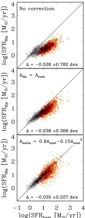
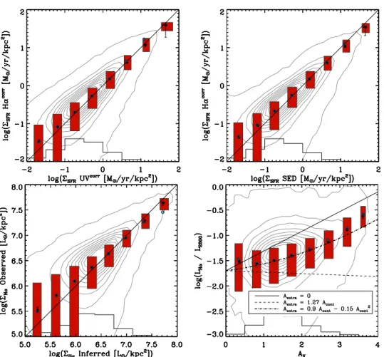
Figure 2.Comparison of Hα-based SFR estimates to the reference ladder of SFR indicators from Wuyts et al. (2011b), in order of priority based on UV +Herschel/PACS, orSpitzer/MIPS 24μm, orU-to-8μm SED modeling. We mark UV+IR-based SFRs in red and indicate galaxies without IR detections with gray circles. Crowded regions of the diagram are displayed with a darker hue. HαSFRs need to be corrected for dust extinction to avoid underestimates (top panel). Applying an extinction correction corresponding to what is inferred from SED modeling is insufficient (middle panel). Accounting for extra extinction toward Hiiregions, we find a good correspondence to the reference SFRs with modest scatter and without systematic offsets (bottom panel). (A color version of this figure is available in the online journal.)
no IR detection is available (see Section2). Figure2contrasts Hα-based SFRs from 3D-HST to the reference SFRs. The top panel iterates the obvious necessity for dust corrections to the Hα emission. The large sample statistics exploited here also demonstrate unambiguously the presence of additional extinc-tion toward the nebular regions (middle panel of Figure2, where
Aextra=0 is assumed and significant systematic underestimates
for highly star-forming systems are evident). Finally, the bottom panel of Figure2shows the improved agreement between the
SFR measurements once differential extinction is accounted for. The adopted prescription,
Aextra=0.9Acont−0.15A2cont, (2)
yields a scatter of 0.227 dex and a negligible systematic offset of−0.035 dex. We note that applying the Calzetti et al. (2000) prescription for extra extinction (corresponding to AHα =
Acont/0.44, or equivalentlyAextra=1.27Acont) leads to a slightly
higher systematic offset of 0.066 dex and produces a larger scatter of 0.284 dex. If we were to adopt the Calzetti et al. (2000) prescription, all objects with high inferred AV values
from broadband SED modeling would have dust-corrected Hα SFRs systematically in excess of the reference indicator. We note that the need for an extra extinction correction is a result that is largely driven by the more actively SFGs. For most of them, UV+IR (i.e., bolometric, rather than dust corrected) measurements of the SFR are available. Those galaxies that lack IR detections in the CANDELS/3D-HST fields generally suffer less obscuration and are therefore less sensitive to the precise dust correction applied (although applying a constant Aextra,
even to sources withAcontnear zero, would lead to overestimated
HαSFRs at the low-SFR end).
3.3.3. Hα/UV Ratios
We now assess the validity of the calibration to correct Hα for dust extinction (Equation (2)) by considering an independent dust-sensitive diagnostic, namely the Hα/UV luminosity ratio. Here, we define the UV luminosity as the rest-frame luminosity L2800 ≡ νLν(2800 Å), which we compute with EAZY. In
principle, the LHα/LUV ratio is not uniquely dependent on
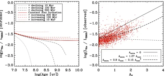
dust extinction, but may also vary among galaxies that differ in their relative number of O and B stars due to differences in the star formation history or initial stellar mass function (see, e.g., Meurer et al. 2009). The reason is that the Hα emission is powered by the ionizing radiation from O stars (with typical lifetimes of ∼7 Myr), while the rest-frame UV light receives its major contributions from both O and B stars (i.e., stellar lifetimes up to ∼300 Myr). The left-hand panel of Figure 3 visualizes the evolution in LHα/LUV for a set of
BC03 stellar populations models with varying star formation histories. Here, we calculated the intrinsic Hαluminosities from the rate of H ionizing photons in the BC03 models. Applying the recombination coefficients for case B from Hummer & Storey (1987) for an electron temperature ofTe =104K and density
ofne=104cm−3, this gives
log(LHα[erg s−1])=log(NLyc[s−1])−11.87 (3)
whereNLycis the production rate of Lyman continuum photons
from the stars. It is noticeable that, except for very young stellar populations or abruptly declining star formation histories, the balance between the intrinsic (i.e., unattenuated) Hαand UV emission quickly converges to a value of around−1.7. We re-mind the reader that the frequently used Kennicutt (1998) SFR conversions, which assume a 100 Myr old constant star forma-tion populaforma-tion, correspond to the same ratio. In the following, we adopt log(LHα/LUV) = −1.7 as the expected intrinsic
ra-tio in the absence of dust. We make the plausible assumpra-tion that any observed variation inLHα/LUV will be dominated by
Figure 3.Left: dependence of the intrinsic (i.e., extinction free) Hα/UV (2800 Å) luminosity ratio on age since the onset of star formation for a range of star formation histories (exponentially declining or increasing and constant star formation). The Kennicutt (1998) SFR conversions from Hαand UV assume a population with constant star formation ongoing for 100 Myr. Right: given a stellar population as assumed by Kennicutt (1998), the observed Hα/UV luminosity ratio depends on the visual extinctionAV as indicated by the black lines, which correspond to three different models for extra extinction toward Hiiregions: no extra extinction (solid), double Calzetti (AHα=Acont/0.44; dashed), and limited extra extinction (Equation (2); dash–dotted). The latter model best describes the locus of observed galaxies (small red dots).
(A color version of this figure is available in the online journal.)
It is then possible to represent different prescriptions for extra extinction toward the nebular regions by lines in a diagram ofLHα/LUV versusAV (right-hand panel of Figure3). In the
absence of extra extinction, the Hα/UV ratio increases linearly with increasing AV, while it remains relatively constant (in
fact drops slightly) with increasingAV for a so-called “double
Calzetti” prescription. Neither prescription provides a satisfying description of the locus of observed 3D-HST galaxies in the diagram (red symbols). Instead, the curve corresponding to Equation (2) matches the data well. In Section 5.2, we will demonstrate that our prescription for Hαdust corrections, the associated dependence of Hα/UV ratios on extinction, and in general the above geometrical picture of a two-component dust distribution still holds on the kiloparsec scale resolution of theHSTdata. A direct implication of the observed increase in Hα/UV ratios withAV is the fact that Hαluminosities are less
sensitive to dust than UV luminosities.
Finally, as an additional verification of the applicability of our Hα dust prescription (Equation (2)), we repeated the comparison of SFR estimates and our analysis of theLHα/LUV
versusAV diagram for the upper and lower tertiles of the axial
ratio distribution of our galaxies separately. We confirm that a good correspondence remains, with only marginal systematic shifts. While the sense of the minor inclination dependence qualitatively agrees with the findings by Wild et al. (2011) for nearby galaxies (edge-on systems requiring relatively less extra extinction because a larger fraction of the obscuring column toward nebular regions is contributed by diffuse dust), we opt not to introduce an extra inclination term in our prescription, given its small amplitude compared to the scatter among galaxies of a given axial ratio.
4. CASE EXAMPLES
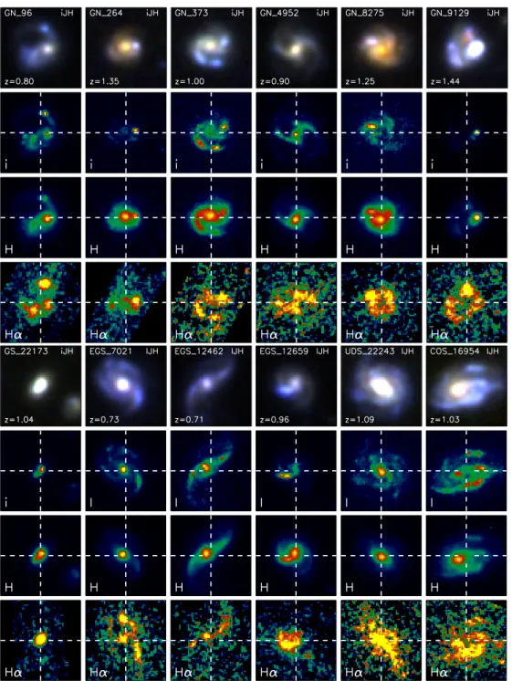
Before quantitatively analyzing the Hα properties of our sample of massive z ∼ 1 SFGs, it is insightful to visually inspect a set of case examples. Figure4 shows a subset of 12 SFGs, illustrating the diversity in size, color, and morphology represented in the sample. Despite their diverse appearance, some key trends that also characterize the sample as a whole can be noted.
First, the central regions of most (and in particular the larger) galaxies are more pronounced in the observedHthan in theI band. This reflects the negative color gradients (red cores) found in previous work and more compact stellar mass distributions based thereupon (e.g., Szomoru et al.2011,2013; Wuyts et al.
2012; Guo et al. 2012). Second, the I-band images appear clumpy or feature spiral signatures more frequently than the rest-opticalH-band images, echoing findings that the clumps/ spiral arms are bluer than the underlying disk (Wuyts et al.2012; Guo et al.2012).
New with respect to these previous studies is that we can now also contrast the Hαmorphologies to the short- and long-wavelength broadband morphologies. A visual inspection tells us that overall the Hαmorphologies resemble more closely the I-band images than theH-band surface brightness distributions. Both the rest-UV light and Hαemission are dominated by the youngest stellar populations, unlike the rest-optical emission to which the bulk of the stars (including older populations) contribute. It is, however, not a trivial observation because of the different wavelengths probed and dust effects discussed in Section 3.3. Moreover, exceptions exist in which the Hα morphology does not trace theI-band light. For example, the I-band emission of GN_9129 is entirely dominated by a clump that is not the most prominent Hαclump in the object. In addition, for the smaller galaxies we are hard-pressed to make a statement on whether the visual morphological match of the Hαmap is closer to I than to the H band. Galaxies such as GS_22173 just appear compact in all bands considered. These results are reminiscent of the conclusions drawn by Nelson et al. (2012) on the basis of a sample of 56 EW-selected galaxies in 3D-HST.
5. RESULTS
5.1. HαEmission Traces the Rest-UV Better Than the Rest-optical Light
Figure 4.Gallery of case examples from the massivez∼1 SFG sample. PSF-matched three-color postage stamps sized 3.4×3.4 are composed ofi775J125H160 for galaxies from the GOODS fields, andI814J125H160for galaxies in EGS/UDS/COSMOS. Below, we show the surface brightness distributions inI,H, and Hα, respectively (at natural resolution, with a slight smoothing applied to the Hαmaps for visualization purposes). Blue, star-forming regions present in theIband generally dominate the Hαemission as well. Central peaks in surface brightness (i.e., “bulges”) appear more prominently in theHband.
(A color version of this figure is available in the online journal.)
astrometric frame of the CANDELS broadband images. This accounts for uncertainties in the position of the grism spectra on the detector and degeneracies between on the one hand the systemic redshift and on the other hand morphological k-corrections between the Hαline map and the galaxy’s F140W light distribution that was used as template in the redshift determination. For each band, we adopted the shift leading to the largest correlation coefficient, in most cases limited to 0–3 pixels.16 The ratio ofI-to-Hband correlation coefficients then serves as a quantitative measure of how much better the
16 One pixel corresponds to 23 Å in wavelength, and 0.06 spatially.
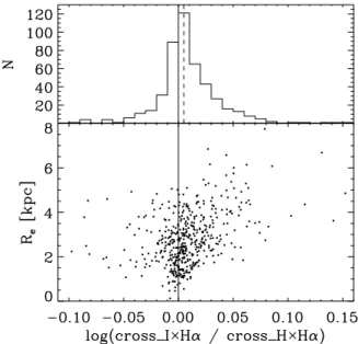
Figure 5.Top: histogram of the ratio of cross-correlation strengths between the Hα and I-band surface brightness distribution and the Hα- and H -band surface brightness distribution, respectively. The vertical dashed line marks the median. The distribution is asymmetric with a tail toward positive values of log(cross I/cross H), representing objects whose Hαprofiles greater resemble those observed in theIband than in theHband. Bottom: the closer correspondence between the Hα- and I-band images is most prominent for the larger galaxies in our sample (withRebeing the effective radius measured by fitting a S´ersic profile to theH-band light profile). More compact galaxies generally look similar at all considered wavelengths (I,H, and Hα).
SFGs at z ∼ 1, with Re > 5 kpc, this fraction increases
further to above 90% (see, e.g., EGS_7021 and COS_16954 in Figure 4). We stress that the above statements on the resemblance between line emission maps and broadband images of different wavelengths are of a comparative nature. Substantial pixel-to-pixel variations exist in the flux ratio between Hαand any single broad band (even at short wavelengths), preventing a simple scaling from a monochromatic broadband image to Hα without additional information. In the next section, we explore how multi-wavelength broadband information improves this situation and furthermore allows us to dust correct Hα maps to star formation maps.
5.2. Comparing Resolved Broadband and Emission-line Diagnostics
5.2.1. Resolved Dust and SFR Calibrations
We now proceed to translate the direct observables (i.e., sur-face brightness profiles in Hα and multiple broad bands) to more physically relevant quantities following the resolved SED modeling and Hαextinction correction methodologies outlined in Section3. Figure6 contrasts various Hα-based diagnostics to stellar population properties inferred using broadband infor-mation alone. We place each spatial bin of each galaxy in the respective diagrams and consider the locus of observed points, marked by contours. Due to noise, some individual spatial bins have negative Hα fluxes and therefore do not appear in the plot. These pixel bins are, however, included in the binned me-dian and central 50th percentile statistics marked in red. In a resolved analogy to Figure 3, we confirm the distribution of observed Hα/UV ratios to relate to the visual extinction AV
inferred from resolved SED modeling as would be expected from Equation (2). In contrast,Aextra=0 orAextra=1.27Acont
do not reproduce the observed locus of galaxy spatial bins in
the diagram. Consequently, it comes as no surprise that, when applying dust corrections according to Equation (2) to the Hα emission, we find the Hα-based ΣSFR to correspond well to
dust-corrected UV-based estimates. To compute the latter, we converted the rest-frame 2800 Å luminosity L2800 to an
unob-scured UV SFR based upon the Kennicutt (1998) conversion
SFRUV,uncorrected=3.6×10⁻¹⁰L2800/Land finally applied an
extinction correction based on the broadband SED modeling, which assumed a Calzetti et al. (2000) attenuation law. Since the visual extinction appears in the quantities on both axes of the Hα- versus UV-based dust-correctedΣSFR, we also show that a
strong correlation remains when plotting the directly observed Hαluminosity surface density (i.e., uncorrected for dust) as a function of it would be inferred to be on the basis of the available broadband information.
5.2.2. The Resolved Main Sequence of Star Formation
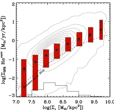
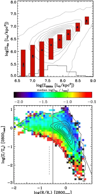
Using the analysis of SFR estimates and dust treatment, we now turn to Figure7, which contrasts the Hα-based SFR surface density of individual sub-galactic regions to the surface density of stellar mass present at the respective location in the galaxy. As such, the diagram can be regarded as a spatially resolved version of the SFR–mass plane that has been the focus of many galaxy evolution studies in recent years. We find a relation between the star formation activity and amount of assembled stellar mass to be present for sub-regions within galaxies, as is the case for galaxies as integrated units. Similar to the well-established, galaxy-integrated main sequence of star formation, we observe a near-linear slope:
log(ΣSFR[Myr−1kpc−2])= −8.4 + 0.95 log(Σ∗[Mkpc−2]), (4) as fit to the spatial bins with log(Σ∗) < 8.8. Akin to galaxy-integrated observations at the high-mass end by, e.g., Whitaker et al. (2012), the “resolved main sequence” shows a tendency to flatten at the high stellar surface mass density end. Consequently, a linear fit to all spatial bins spanning the entire range in Σ∗, yields a slightly shallower slope, of 0.84. We conclude that, even if global galaxy properties such as halo mass or cosmological accretion rate drive the stellar build-up within galaxies, this happens in such a way that on average the ongoing and past-integrated star formation activity track each other on sub-galactic as well as galactic scales. This is at least the case down to the∼1 kpc scales probed at the WFC3 resolution, albeit with a significant scatter and possible exceptions (i.e., reduced specific SFRs) at the highest stellar surface mass density end.
In the remainder of the paper, we will investigate the deviation from a perfectΣSFR ∝ Σ∗ relation more closely and illustrate
where variations in local specific SFRs occur spatially within galaxies. Analogous to the galaxy-integrated main sequence of star formation, the clumps/spiral arms featuring excess star formation with respect to the smooth underlying disk (Section 5.3.1) can be thought of as sub-galactic equivalents to the starbursting outliers above the main sequence.
5.3. Resolved HαProperties in the Two-dimensional Profile Space
5.3.1. The Nature of Excess Surface Brightness Regions
Figure 6.Comparison of resolved galaxy properties based on Hαvs. resolved stellar population properties derived from broadband information alone. Contours indicate the locus of all spatial bins of the galaxies in our sample. Red bars with black dots mark the central 50th percentile and median, respectively. With open blue circles, we mark the median results for the subset of galaxies in the GOODS fields, where the high-resolution multi-wavelength sampling is best, with seven bands. Black histograms illustrate the distribution of spatial bins. The dust-corrected HαSFRs of individual spatial bins within galaxies compare favorably to estimates from the UV or SED modeling (top panels). Bottom left: a good correlation remains when plotting the directly observed Hαluminosity surface density (i.e., without dust correction) as a function of what would be inferred on the basis of broadband information, demonstrating theΣSFRagreement is not just due to the appearance ofAV in the quantities on both axes. Bottom right: the Hα/UV luminosity ratio of individual spatial bins within galaxies shows a similar dependence on visual extinction as observed in a galaxy-integrated sense in Figure3.
(A color version of this figure is available in the online journal.)
enhanced level of star formation with respect to the underlying disk. Given short timescales for these spatial fluctuations in local star formation, the same substructure is not necessarily present in the distribution of stellar mass as would be expected if the observed irregular morphologies were all due to merging activity.
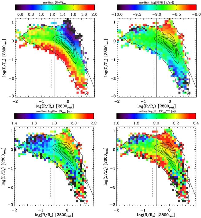
Following Wuyts et al. (2012), we employ co-added nor-malized profiles to infer the characteristic star formation prop-erties of pixels belonging to the galaxy’s central regions, off-center clumps (or spiral arms), and the (interclump) outer disk (Figure8). In each of these diagrams, we consider all spatial bins of all 473 SFGs as being part of one meta-galaxy, repre-senting the massive SFG sample as an ensemble whose resolved stellar populations we then dissect. We apply identical criteria to Wuyts et al. (2012) in order to separate spatial bins belonging to the three regimes:
[center] log(R/Re)<−0.5 (5)
[disk] log(R/Re)>−0.5 & (6)
log(Σ/Σe)<0.06−1.6 log(R/Re)−log(R/Re)2
[clump] log(R/Re)>−0.5 & (7)
log(Σ/Σe)>0.06−1.6 log(R/Re)−log(R/Re)2,
whereΣ/Σeis the rest-frame 2800 Å surface brightness
normal-ized by the average surface brightness level within the effective radiusRe. As in Wuyts et al. (2012), we define radii on
ellip-tical apertures whose center and axial ratio are derived from the stellar mass maps. Since the distance from the center of a spatial bin to the center of mass of the galaxy can in principle be arbitrarily small, we note that the precise galactocentric radii at small log(R/Re) −0.5 becomes meaningless. Throughout
the paper, we therefore treat all pixels with log(R/Re)<−0.5
as belonging to the inner regions of galaxies without further regard to their precise value of R/Re. In the top panels of
Figure 8, we first demonstrate that the conclusions drawn by Wuyts et al. (2012) based on broadband information alone also apply to our Hαsample at 0.7 < z <1.5. Off-center clumps identified at short wavelengths by an excess in surface brightness are characterized by bluer rest-optical colors than the underlying disk. Taking one step further away from the direct observables, stellar population synthesis modeling of the multi-wavelength HSTcolors implies that they correspond to sites of enhanced star formation activity (SSFR) with respect to the underlying disk.
Figure 7.Equivalent to the so-called “main sequence of star formation” for galaxies; resolved subregions within galaxies exhibit a correlation between the level of ongoing star formation and the surface density of assembled stellar mass (plot style as in Figure6). For reference, the dashed line marks the slope of the galaxy-integrated main sequence from Whitaker et al. (2012).
(A color version of this figure is available in the online journal.)
bulk of the stars present in the galaxy. As the emission line and continuum are measured at the same wavelength and both components are subject to the attenuating column of diffuse dust in the interstellar medium of the galaxy, extinction effects due to the latter divide out. We observe the Hα EW to be higher in the clumps/spiral arm regions (with a median rest-frame EWHα ≈ 100 Å) than in the underlying smooth disk
(EWHα ∼70 Å), while the lowest EWs are measured at small
radii. The latter are associated with the regions of highest stellar surface mass density and are related to the flattening slope of the resolved main sequence at highΣ∗(see Section5.2.2). The implications of the radial trends will be discussed in depth in a forthcoming comprehensive overview of Hαand star formation profiles as a function of galaxy mass and SFR by E. Nelson et al. (in preparation). Here, we consider in more detail the characteristic trends with surface brightness at a fixed radius. As discussed in Section3.3.2, an additional extinction correction to account for the obscuring material in birth clouds from which the Hα line emission originates is required for the EW to be an unbiased proxy of the star formation activity. In the bottom right panel of Figure8, we apply this correction and find an excess in the clumps’ intrinsic HαEW by 25% in the median with respect to the underlying disk (i.e., interclump regions) at the same galactocentric radii. We note that the median excess between the EW of clump and disk pixels does not reflect the full dynamic range in rest-2800 Å surface brightness variations at a given radius and the extent of the associated trend in the Hα EW. The reason is that the distribution of disk and especially clump pixels is dominated in numbers by pixels that lie close to the dividing line between the two regimes (see contours). The color coding in Figure8illustrates that excess EWs by factors of two to three are commonly observed when considering the full range of surface brightness levels observed at a given radius.
In order to address whether the clump and spiral arm regions selected through our methodology differ in other aspects than
star formation activity from the diffuse outer disk, we now inves-tigate the relation between the Hαand rest-2800 Å luminosity surface densities (both uncorrected for extinction; Figure9, top panel). As already hinted at by the similar morphological ap-pearance of our galaxies in Hαand ACS imaging (Sections4
and5.1), the UV and HαSFR tracers correlate strongly, both spatially and in amplitude. Their measured luminosity surface densities prior to any dust correction, however, do not follow a relation with a unity slope. Instead, the formal best-fit linear relation is
log(ΣHα[Lkpc−2])=0.2 + 0.8 log(Σ2800[Lkpc−2]). (8)
Two potential contributors to the deviation from a unity slope, scatter around the relation, and, in more general terms, behind variations in Hα/UV luminosity ratios, are dust extinction and variations in the star formation history (see Section3.3). While both Hα and UV light are tracing young stellar populations, they probe recent star formation over different timescales (around 10 Myr and 100 Myr, respectively). The UV and Hα radiation are furthermore emitted at different wavelengths, and, moreover, continuum and nebular emission may travel different paths through the galaxies’ dusty interstellar medium. The combination of these effects leads to systematically larger Hα/UV ratios with increasing extinction compared to the intrinsic (i.e., dust-free) ratio.
Evaluating the spatial variation of Hα/UV ratios within our z∼1 SFGs (Figure9, bottom panel), we find the clumps/spiral features to correspond to lowerLHα/LUV than the underlying
disk at the same radius. Three effects can potentially contribute to this trend. The first relates to measurement uncertainties rather than physics. If the true Hα/UV ratio were constant across galaxies, measurement errors would preferentially push those spatial bins over the clump selection threshold for which Σ2800 is overestimated. Since the 2800 Å luminosity appears
in the denominator, the measured Hα/UV ratio for those bins would consequently be lower than the true value. While possibly contributing in a minor way, this effect is unlikely to be by itself responsible for the observed trend, given the small uncertainty onΣ2800(see theAppendix) and the fact that the clumps are also
confirmed to be physically distinct from the underlying disk in quantities that are measured independently of the 2800 Å luminosity (e.g., the HαEW).
A more physical interpretation is that the excess surface brightness regions selected from rest-UV ACS imaging are not only regions characterized by enhanced star formation, but preferentially those local enhancements in star formation that are the least obscured. Speculatively, outflows driven by the enhanced star formation density in “clumps” (see, e.g., Newman et al.2012) may be responsible for the clearing of gas and dust toward these sightlines.17
Finally, we cannot exclude that recent variations in the star formation history contribute to the lower Hα/UV ratios of clumps as well. We note, however, that a recent upturn of the SFR in spatial bins that are classified as clumps or spiral features would lead to elevated Hα/UV ratios (i.e., relatively more O stars compared to the number of B stars), the opposite of what is observed. Interpreting the Hα/UV ratios in terms of changes in the star formation history would therefore invoke a rapidly declining SFR (see Figure 3) and consequently a
Figure 8.Co-added normalized rest-UV surface brightness profile of the SFGs in our sample. The vertical dashed line indicates the typical resolution. Contours denote the density of spatial bins. The top panels are color-coded by purely broadband-based quantities, namely the rest-frame optical color (U−V)rest(top left) and the specific SFR inferred from resolved stellar population modeling (top right). The color-coding in the bottom panels marks the Hαrest-frame equivalent width as observed directly (bottom left) and after correction for extra extinction toward the nebular regions (bottom right). Solid lines separate the central, outer disk, and clump/spiral arm regimes. Spatial bins in the clump/spiral arm regime are characterized by bluer broadband colors and higher HαEWs, consistent with the elevated SSFR with respect to the underlying disk inferred from the resolved SED modeling.
(A color version of this figure is available in the online journal.)
prior (possibly very short-lived) phase of even more intense star formation. The latter phase necessarily would have to be embedded, since otherwise it would itself be picked up by the UV clump selection. As such, both physical explanations could go hand in hand, in a scenario where outflows quickly clear the gas and dust from clumps, simultaneously reducing their star formation activity and obscuration, and consequently lowering the observed Hα/UV ratio. If true, this would imply that resolved observations at longer wavelengths with ALMA or Plateau de Bure Interferometer (PdBI)/NOEMA may reveal new/different clumps that correspond to an earlier, embedded evolutionary stage of star-forming regions.
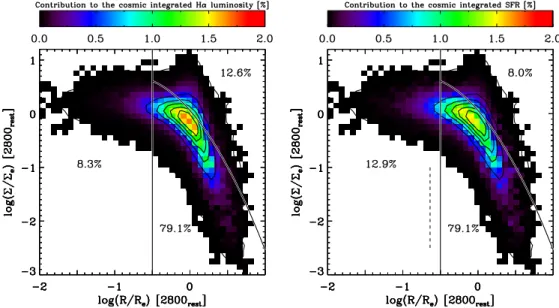
5.3.2. Where Do the Stars Form inz∼1SFGs?
Figure 9.While the Hαluminosity surface density correlates with the rest-frame 2800 Å luminosity surface density of individual bins (top panel), variations in the Hα/UV luminosity ratio are present and show a systematic dependence on the spatial location of pixels within the galaxies (bottom panel; identical in style to Figure8). The reduced Hα/UV luminosity ratios of clumps with respect to the fainter interclump regions may arise from spatial variations in effective attenuation (i.e., reduced dust extinction toward those sites of enhanced star formation where the rest-UV surface brightness is observed to peak). (A color version of this figure is available in the online journal.)
it is clear that the vast majority of the Hα emission arises from the disk component.18A similar conclusion can be drawn from the breakdown of the rest-frame 2800 Å luminosity budget with modest differences that can be understood from the trends described in Section5.3.1and specifically Figure9. The clump pixels account for 18% of the integratedL2800 luminosity. It
should be noted that the precise percentages quoted above depend significantly on the adopted dividing lines between the regions (Equations (5)–(7)), and the fractional contribution of
18 Here, we accounted for the masked pixels that could potentially be affected by [Sii] line emission (see Section3.2), to avoid a biased weighting of different radial bins.
excess surface brightness regions should be regarded as coming from bright clumps and spiral features that show sufficient contrast with respect to the extended smooth disk to be detected at the kiloparsec resolution of WFC3. For example, if we were to lower the dividing line between the disk and clump regions by 0.2 dex, bringing it close to the peak of the contours in Figure10, the fractional contribution of clumps in this adjusted definition would be 30% to the Hαluminosity and 23% to the Hαderived SFR. The latter percentages can be interpreted as a rough estimate of the upper limit on the fractional contribution by UV bright clumps.
As discussed extensively in Section3.3.2, the Hαluminosity is not a direct tracer of the total on-going star formation since part of the ionized gas emission is filtered out by the intervening obscuring material. As discussed by Wuyts et al. (2012), SFGs feature radial gradients in dust extinction. This results in an enhanced contribution of the inner (log(R/Re)<−0.5) regions
of the galaxies to the integrated SFR budget of our sample: 12.9% when computing the budget based on dust corrected Hα emission. A similar contribution of 14.8% is obtained from broadband SED modeling. Wuyts et al. (2012) found similar fractional contributions for their mass-complete sample ofz∼1 SFGs, confirming that our Hαsample is not subject to significant biases in this regard. Using broadbandHSTimaging, Wuyts et al. (2012) also extended the analysis toz= 2.5, finding that the fractional contribution of clumps to the integrated SFR of SFGs increases to∼20% atz∼2.
We conclude that most stars being formed during and since the peak of cosmic star formation are born in a disk component. This result is consistent with the analysis of SFR profiles presented for a smaller 3D-HST sample by Nelson et al. (2013) and is in line with a larger body of work based onHSTimaging (e.g., F¨orster Schreiber et al.2011a,2011b; Wuyts et al.2011b,2012; Guo et al. 2012) and ground-based kinematic measurements (e.g., Genzel et al.2006; F¨orster Schreiber et al.2009; N. M. F¨orster Schreiber et al. in preparation; Lemoine-Busserolle & Lamareille2010; Wisnioski et al.2011; Epinat et al.2012).
6. SUMMARY
We combined CANDELS high-resolution multi-wavelength imaging on kiloparsec scales of a sample of 473 SFGs at 0.7< z <1.5 with maps of the Hαline emission from 3D-HST. Together, the CANDELS + 3D-HST data shed light on where within galaxies new stars are being formed and in which amounts stellar mass has been assembled at each location throughout their history prior to observation. As such, the present study builds on earlier work from 3D-HST (Nelson et al.2012,2013) and CANDELS (Wuyts et al.2012). Compared to the former study, we expand the sample to a more representative subset of all massive (log(M∗) > 10) SFGs at z ∼ 1, while compared to the latter, we extract sources from all five CANDELS/3D-HST fields instead of one.
Figure 10.Co-added normalized rest-UV surface brightness profile of the SFGs in our sample (identical in style to Figure8). The color-coding of each bin in the diagram indicates the percentage of the total integrated Hαluminosity (left panel) or dust-corrected SFR based thereupon (right panel) summed up from all massive SFGs in our sample, originating from the respective region in 2D profile space (i.e., galactocentric radius and rest-2800 Å surface brightness level). Differences between the fractional contribution to the cosmically integrated Hαluminosity and SFR arise from inhomogeneous dust distributions within galaxies: thicker dust columns toward the center and slightly reduced obscuration of the rest-UV-selected clumps. The vast majority of newborn stars inz∼1 galaxies are being formed in the disk.
(A color version of this figure is available in the online journal.)
nearby starburst galaxies. Our findings fit in the context of a two-component geometrical dust model in which the ionized gas emission surrounding young star-forming regions is obscured by dust from the birth cloud itself in addition to the column of diffuse material spread throughout the galaxy that also affects the bulk of galaxy light emitted by older stars (see also Charlot & Fall2000; Wild et al.2011; Pacifici et al.2012; Chevallard et al.2013). As an independent test, we confirmed that this prescription for extra extinction toward Hiiregions reproduces the relation between the observed Hα/UV luminosity ratio and the effective visual extinction inferred from broadband SED modeling. The fact that the observed Hα/UV luminosity ratio rises with increasing visual extinction directly implies that Hα is a less dust-sensitive SFR tracer than UV emission.
From our resolved stellar population analysis, we draw the following conclusions.
1. The Hα morphologies of z ∼ 1 SFGs resemble more
closely the ACSI-band morphologies than those observed in the WFC3 H band, particularly in the case of large galaxies.
2. The Hαand rest-frame 2800 Å luminosities correlate on a pixel-by-pixel basis, and after proper dust corrections are applied, the SFR estimates based thereupon are internally consistent. The Hα/UV luminosity ratios of individual spatial bins also relate to the visual extinction inferred from multi-bandHSTphotometry in a manner that is consistent with the applied correction for extra extinction toward the Hiiregions.
3. We find evidence for the existence of a resolved main se-quence of star formation: the rate of ongoing star formation per unit area tracks the amount of stellar mass assembled over the same area. Its near-linear slope is consistent with the one measured for the galaxy-integrated main sequence, including an apparent flattening at the high-mass density end, associated with the low-EW inner regions of the most massive galaxies.
4. Off-center clumps (or spiral features that show up similarly as regions with excess surface brightness) are character-ized by enhanced Hα EWs, bluer broadband colors, and correspondingly higher SSFRs than the underlying disk, implying that they are a star formation phenomenon. Phys-ically, they may correspond to regions with elevated gas fractions and/or star formation efficiencies (Tacconi et al.
2013), where part of the global gas disk collapsed through gravitational instabilities (see, e.g., Bournaud et al.2008; Genzel et al.2008; Dekel et al.2009), although atz∼1 sec-ular processes on longer timescales, such as spiral density waves, are also likely to contribute. In an integrated sense, however, the contribution of excess surface brightness re-gions to the total amount of star formation taking place withinz∼1 SFGs is limited to 10%–15%, depending on the tracer. Most stars being formed betweenz =1.5 and z=0.7 are formed in the disk component (see also F¨orster Schreiber et al.2009; N. M. F¨orster Schreiber et al. in prepa-ration; Nelson et al.2013). Wuyts et al. (2012) demonstrated that this conclusion holds out toz∼2, where the fraction of total star formation in off-center clumps increases, but does not exceed∼20%.