Modeling Crack Patterns by Modified STIT Tessellations

(1)

MODELING CRACK PATTERNS BY MODIFIED STIT TESSELLATIONS

ROBERTO

LE

ON

´

1,

WERNER

NAGEL

B,2_,

_JOACHIM

_OHSER

3 _AND

_STEVE

_ARSCOTT

4 1_{Universidad Andr´es Bello, Facultad de Ingenier´ıa, Quillota 980, Vi˜na del Mar, Chile;}2_{University of Jena,}

Institute of Mathematics, 07737 Jena, Germany;3University of Applied Sciences, Department of Mathematics and Natural Sciences, Schöfferstr. 3, 64295 Darmstadt, Germany;4Institut d’Electronique, de Microélectronique et de Nanotechnologie (IEMN), CNRS, The University of Lille, Cité Scientifique, 59652 Villeneuve d’Ascq, France

e-mail: [email protected], [email protected], [email protected], [email protected]

(Received August 21, 2019; revised November 29, 2019; accepted December 2, 2019)

ABSTRACT

Random planar tessellations are presented which are generated by subsequent division of their polygonal cells. The purpose is to develop parametric models for crack patterns appearing at length scales which can change by orders of magnitude in areas such as nanotechnology, materials science, soft matter, and geology. Using the STIT tessellation as a reference model and comparing with phenomena in real crack patterns, three modifications of STIT are suggested. For all these models a simulation tool, which also yields several statistics for the tessellation cells, is provided on the web. The software is freely available via a link given in the bibliography of this article. The present paper contains results of a simulation study indicating some essential features of the models. Finally, an example of a real fracture pattern is considered which is obtained using the deposition of a thin metallic film onto an elastomer material – the results of this are compared to the predictions of the model.

Keywords: fracture pattern, geometry-statistics, Monte Carlo simulation, random tessellation, STIT tessellation.

INTRODUCTION

The main purpose of the paper is to develop a variety of mathematical models and modeling tools for the simulation of crack patterns. Our approach is based on ideas of stochastic geometry, in particular of random tessellations (random mosaics). We aim at providing parametric models which allow for a quantitative description of some classes of crack patterns.

The literature contains numerous examples of cracking and fracturing in fields ranging from geology and materials science to soft matter and nanotechnology. Often, these papers focus on the genesis and physics of an individual crack, e.g., Thouless et al. (1987); Hutchinson and Suo (1991). However, there are also approaches to whole crack

patterns, seee.g., Xia and Hutchinson (2000); Iben and O’Brien (2006); Hafveret al.(2014); Boulogneet al.

(2015); Seghir and Arscott (2015); Nandakishore and Goehring (2016); Kumar et al. (2017). Furthermore, also networks of roads are modeled as tessellations, see

e.g., Yuet al.(2014).

Being able to model and predict large surface cracking would be beneficial to those working in the above mentioned applied fields. This is the reason why we have developed the “Crack Pattern Simulator” (Le´on, 2019).

We consider tessellations of the Euclidean plane

R2 which are defined as a collection of convex

polygons partitioning the plane. The polygons forming a tessellation are called cells.

The STIT tessellations – tessellations that are

STable under the operationITeration of tessellations – were invented and first introduced in Nagel and Weiß (2005). This stochastic stability is an essential property which also allows for many theoretical results.

STIT tessellations belong to a class of random tessellations which are generated by consecutive division of their cells. There are two features of such a cell division process, as they were systematically introduced in Cowan (2010):

L The rule for the random lifetime of a cell,i.e., the time between the birth of a cell by division of a mother cell, and the division of the cell.

D The rule for the randomdivisionof a cell at the end of its lifetime.

In these models it is assumed that the lifetime and the division of an extant cell only depend on the cell itself, and neither on the adjacent cells nor on the history of the division process.

(2)

The realization of a planar STIT tessellation in Fig. 1 suggests that it can be a potential model for crack or fracture patterns as they arise in materials science, nanotechnology, geology, or drying soil patterns.

However, already tentative studies in Nagelet al.

(2008) or Mosser and Matth¨ai (2014) indicated that for several patterns the STIT tessellations are not appropriate. This is not surprising because the STIT model emerged from purely mathematical ideas. Thus, an adaption of the cell division model to data of such fracture patterns is necessary. We have chosen a more “phenomenological approach”, i.e., we aim to model the geometric appearance, not focusing on the physics of crack formation.

In the present paper we suggest three modifications of the STIT model which are motivated by observations of fracture patterns. Briefly, the ideas are: when a cell is divided, the dividing line tends to be closer to the center of the cell than to the fringe of the cell. Therefore, we suggest the division rule D-GAUSS, which is introduced below.

Furthermore, the lifetime of a cell seems to depend rather on its area than on its perimeter, i.e., the probability that a cell is divided at a certain moment is larger the larger its area is. This motivates the consideration of L-AREA, where the lifetime of a cell is exponentially distributed with its area as the parameter.

Firstly, we describe the planar STIT tessellation, and then we explain how to generate realizations by Monte Carlo simulation for a given directional distribution of the cell dividing lines.

In the second part of the paper we introduce the mentioned modifications of the STIT model, which are more flexible and thus potentially allow for a better adaption to actual fracture patterns. We present and explain the “Crack Pattern Simulation Tool” (Le´on, 2019) for these models.

Furthermore, some quantitative results of a simulation study are given where we compare the models with respect to certain features.

In the last part of the paper we consider data from a real fracture pattern obtained using the deposition of a thin chromium/gold film onto an elastomer (polydimethylsiloxane, PDMS). A tensile stress in the layered material leads to film cracking. We check how good some statistical parameters can be fitted by the introduced models. A more detailed and thorough modeling will be the subject of forthcoming work.

THE PLANAR STIT MODEL

Denoting byR2the Euclidean plane and byPthe

set of all convex polygons, a subsetT ⊂Pis called a tessellation if

(i) the polygons fill the plane,i.e., [

z∈T

z=R2,

(ii) the polygons do not overlap; more precisely, for allz,z0∈T, ifz=6 z0, then intz∩intz0=/0, where intzdenotes the topological interior ofz, (iii) T is locally finite,i.e., the set{z∈T:z∩C6=/0}

is finite for all compact setsC⊂R2.

A random tessellation is a random variable with values in the set of all tessellations.

A construction of STIT tessellations in bounded windows in a Euclidean space of arbitrary dimension was described in all details in Nagel and Weiß (2005). A global construction, i.e., in the whole space, was given in Meckeet al.(2008).

Here we give a description of the planar STIT tessellations in a convex polygonW ⊂R2, referred to

as the window. Let H denote the set of all lines in the plane. A lineH=H(α,r)∈H is parametrized by

its normal directionα ∈[0,π)and its signed distance

r from the origin, where the distance has a positive sign if the intersection of the line with its orthogonal subspace is in the upper half plane. For a lineH that does not contain the origin, denote byH+andH− the closed halfplanes generated byH, whereH+ contains the origin. Note that in our context the random lines contain the origin with probability zero. For a setB⊂

R2denote by[B] ={H∈H :H∩B6=/0}the set of all

lines intersectingB.

Up to a scaling factor, the distribution of a STIT tessellation is determined by the choice of a directional distribution ϕ, which is a probability distribution on

the interval[0,π). In Eq. 1 and Remark 1 it is explained howϕdetermines the distribution of the lines dividing

the cells. Throughout the paper, it is assumed thatϕ is

not concentrated on a single value. This guarantees that the constructed object is indeed a random tessellation (Schneider and Weil, 2008).

Based onϕ, a translation invariant measureΘon

H is determined, up to a constant factor, by

Z

H f(H)Θ(dH) =

Z

[0,π)

Z

R

f(H(α,r))drϕ(dα)

for any nonnegative measurable function f :H →

[0,∞), see Section 4.4 of Schneider and Weil (2008). An interpretation of this formula and the application in the Monte Carlo simulation is given below.

(3)

values of the signed distances of the tangential lines to z with normal direction α. Formally, h0(z,α) =

min{xcosα +ysinα : (x,y) ∈ z} and h1(z,α) =

max{xcosα +ysinα : (x,y) ∈ z}. Hence, a line

H(α,r) ∈[z], i.e., H(α,r) divides z, if and only if

h0(z,α)<r<h1(z,α).

By b(z,α) = h1(z,α)−h0(z,α) we denote the

value of the width (or breadth) function of z in direction α, i.e., the distance of the two supporting

(tangential) lines tozwhich have the normal direction

α. The maximum width ofz is denoted bybmax(z) =

max0≤α<πb(z,α), and the minimum width of z is

denoted bybmin(z) =min0≤α<πb(z,α).

By1{·}we denote the indicator function which is 1 if the condition in{·}is satisfied, and 0 otherwise. For 0<α0≤πand a convex polygonzwe obtain

Θ({H(α,r)∈[z]: 0<α<α0})

=

Z

[0,π)

1{0<α<α0}b(z,α)ϕ(dα), (1)

and in particular forα0=π

Θ([z]) = Z

[0,π)

b(z,α)ϕ(dα). (2)

Hence, Θ([z]) can be understood as the ϕ-weighted

mean width of z. If ϕ is the uniform distribution

on [0,π) then Θ([z]) =P(z)/π, where P denotes the

perimeter.

For a convex polygon z we define a probability distribution Θ[z] on the set [z] of all lines which

intersectzby

Θ_[z](·) =Θ(· ∩[z])/Θ([z]).

Remark 1 Notice that according to Eq. 1 the directional distribution of a line which intersects a polygon z is notϕ itself, but it isϕ endowed with the

density b(z,α)/Θ([z]). This must be taken into account when a dividing line is generated in the Monte Carlo simulation of a STIT tessellation.

A loose and informal description of the STIT tessellation process is:

L-STIT A cell z, that is born by the division of a larger cell, has a random lifetime which is exponentially distributed with parameter

Θ([z]).

D-STIT At the end of its lifetime,zis divided by a random lineH with lawΘ_[z], independent

of the lifetime, and conditionally independent, given z, of all the dividing lines used before.

To give a formalized definition of the STIT tessellation process, let N denote set of positive

integers and let τ = (τn : n∈N) be a sequence of

independent and identically distributed (i.i.d.) random variables, exponentially distributed with parameter 1. The lifetime of a cell zi will be τi/Θ([zi]), i.e.,

exponentially distributed with parameterΘ([zi]).

LetW ∈P be a convex polygon, referred to as a window. Now we define the process (Yt,W : t>0)

of STIT tessellations, restricted to the windowW. The birth time of a cellzis denoted byβ(z). This definition

looks rather involved but its advantage is that it at once provides an algorithm for the STIT construction.

Definition 1 The STIT tessellation process(Yt,W :t>

0)inW, driven by the measureΘis defined by

(a) Initial setting.

Yt,W ={W} for 0<t <τ1/Θ([W]), β(W) =0

and z1=W .

(b) Recursion.

For t>0, let be Yt,W ={zi₁, . . . ,zin},

i.e., β(zi_k)<t and β(zi_k) +τi_k/Θ([zi_k])≥t for

k=1, . . . ,n.

Define i∗ ∈ {i1, . . . ,in} as the index of the cell

which is the next to be divided, such that

ti∗=β(zi∗) +τi∗/Θ([zi∗])

=minβ(zi_k) +τi_k/Θ([zi_k]):k=1, . . . ,n .

Then Yt,W remains constant until the jump at time

ti∗, when the process jumps, by division of the cell

zi∗ into the state

Yt_i∗,W = ({zi₁, . . . ,zi_n} \ {zi∗})∪ {z2n,z2n+1}

with z₂n=zi∗∩Hi+∗, z2n+1=zi∗∩Hi−∗, where Hi∗

is a random line with lawΘ[z_i∗]and independent

ofτ and conditionally independent, given zi∗, of

the n−1dividing lines used before.

The birth time of the dividing line and of the new cells isβ(Hi∗) =β(z2n) =β(z2n+1) =ti∗.

When zi is divided, the cell zi is replaced by its

two daughter cellszi∩Hi+andzi∩Hi− with birth time

β(zi∩Hi+) =β(zi∩Hi−) =β(zi) +τi/Θ([zi]). At any

fixed timetthe tessellationYt,W is a STIT tessellation,

restricted to the windowW.

A crucial feature of the construction is that the parameter of the exponentially distributed lifetime depends on the size of the cell, expressed by Θ([z]),

(4)

the measure Θ is isotropic, i.e., ϕ is the uniform

distribution on[0,π), the parameter of the exponential

lifetime distribution of a cellzisΘ([z]) =P(z)/π, the

perimeter ofzdivided byπ.

Remark 2 Even if this construction is performed in a fixed and bounded window W it provides a distribution that is spatially consistent in the following sense. Let W0 ⊂W be a convex polygon, (Yt,W0 : t > 0) and

(Yt,W:t>0)the STIT tessellation processes generated

in W0and W , respectively. The symbol=Dstands for the identity of distributions of random variables. Then for all t≥0we have that

Yt,W0 D

={z∩W0:z∈Yt,W,W0∩intz6= /0},

i.e., the restriction of Yt,W to W0 has the same

distribution as Yt,W0. This consistency property yields

that, for any t >0, there exists a spatially stationary (or homogeneous, which means the invariance of the distribution under translations of the Euclidean plane) random tessellation Yt ofR2 such that the restriction

of Yt to W has the same distribution as Yt,W for all

polygons W ∈P.

The process(Yt : t>0)has the following scaling

property

t·Yt D

=Y₁, for allt>0, (3)

wheret·Yt={t·z:z∈Yt}andt·z={tx:x∈z}. This

space-time relation of the STIT tessellation process can be taken into account in the design of a simulation study.

SIMULATION OF PLANAR STIT

TESSELLATIONS

In Le´on (2019) we provide a simulation tool which is described in the present section. The window W

is a square of side length a, which can be chosen in the range a∈N, i.e., a positive integer, e.g., a=1.

Then one has to choose the time tSTOP∈N, at which

the construction stops,e.g.,tSTOP=50. Regarding the

scaling property Eq. 3 it would – theoretically – be sufficient to choosetSTOP=1, but in order to obtain a

reasonable number of cells in a simulation, the value of

tSTOPshould be chosen in an appropriate relation toa.

While the choice of a and tSTOP is an issue of

scaling, the selection of a directional distributionϕfor

the cell dividing lines is an essential ingredient of a STIT tessellation model. By δα we denote the Dirac

measure, concentrated on a single value 0≤α <π,

i.e.,δα(B) =1 if α ∈Band 0 otherwise, for a subset

B⊆[0,π). In the simulation tool one can choose one of the following directional distributions.

List of directional distributions available in the simulation program

ISO: The isotropic distribution, i.e., ϕ is the

uniform distribution on the interval[0,π). DISCR: Adiscrete distributionwith finitely many

directions,i.e.,ϕ=∑ki=1piδαi, 2≤k, with

0≤αi <π and probabilities 0< pi <1,

∑ki=1pi =1. In the generated tessellation

solely segments with normal directions

α1, . . . ,αk appear. Once the number k of

directions is chosen, 2≤k ≤32 in Le´on (2019), one has to insert the values αi as

the radian divided byπ,e.g., the input 0.5 means the angle 0.5π=90◦. And for each αiits probabilitypi has to be inserted.

DDISCR: A disturbed discrete distribution, i.e.,

ϕ = ∑ki=1piδαi

∗ψ, where ψ is the

elliptic distribution with parameter bellip,

see ELLIP below. The ∗ denotes the convolution of measures. This means that a random ‘disturbance’ with an elliptic distribution is added to a direction, which is chosen from a discrete distribution DISCR.

RECT: The discrete distribution with horizontal and vertical directions only, and both with the same probability, i.e., ϕ =

0.5δ0+0.5δπ/2, which is a particular case

of DISCR. The tessellation consists of random rectangles.

DRECT: The discrete distribution RECT which is disturbed by the elliptic distribution ELLIP with parameterb_ellip<1. This is a particular case of DDISCR.

ELLIP: Anelliptic distribution. Consider an ellipse with horizontal half axis of length 1 and vertical half axis of lengthbellip<1. Then

the cumulative distribution function ofϕis

defined as

Fϕ(α) =

area of ellipse sector[0,α]

half area of the ellipse , 0≤α <π.

Notice that for the value bellip = 1 we

obtain the isotropic distribution ISO.

An elliptic distribution can be applied to model a compressed pattern as it appears in geological crack structures or rolled material, cf. Stoyan et al.

(5)

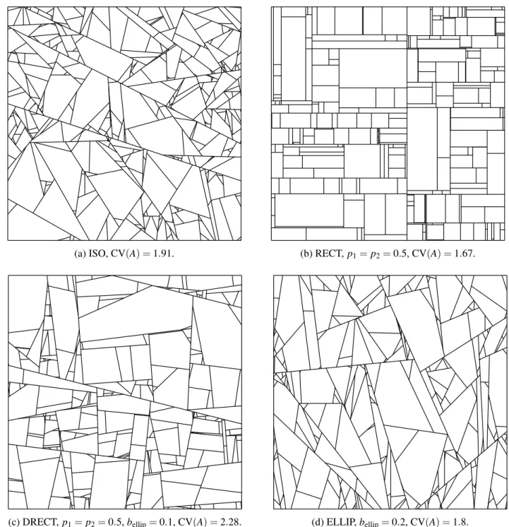
(a) ISO, CV(A) =1.91. (b) RECT,p1=p2=0.5, CV(A) =1.67.

(c) DRECT,p1=p2=0.5,bellip=0.1, CV(A) =2.28. (d) ELLIP,bellip=0.2, CV(A) =1.8.

Fig. 1: Simulations of STIT tessellations with different directional distributions

Fig. 1 shows some examples of simulations of STIT tessellations for different directional distributions.

The algorithm for the Monte Carlo simulation of STIT tessellations follows Definition 1. The integral in Eq. 2, which is needed to determine the lifetime of an extant cellz, is discretized and replaced by a sum using 128 equidistant angles in [0,π). This discretization proved to be sufficiently good for the directional distributions considered. Regarding Remark 1, the simulation of the direction of the line dividing a cell

z requires special attention, because it is not correct

to generate the direction of the dividing line directly fromϕ. In Le´on (2019) we apply a rejection method: For a given cell z, generate a direction α according to ϕ and a random number d which is uniformly

distributed in the interval[h0(z,α),h0(z,α) +bmax(z)].

The simulated line H(α,d) is accepted as a dividing line, ifd<h1(z,α), otherwise it isrejected. Recall that

h0(z,α)< h1(z,α)are the two signed distances of the

tangential lines toz with normal direction α. If for a

(6)

those positions where the line intersects z. Thus, the direction of the accepted dividing line is correctly simulated according to Eq. 1.

MODIFICATIONS OF THE STIT

TESSELLATION

In order to extend the variety of models for crack tessellations, let us reconsider the items L and D given in the Introduction and modify the rules.

L-AREA The lifetime of a cell z is exponentially distributed with parameterA(z), whereA

denotes the area.

D-GAUSS The simulation by the rejection method of the random direction of the cell dividing line is the same as in the STIT model. But then, for a cell z and an accepted direction

α, the signed distance d from the origin is not uniformly distributed in the interval [h0(z,α),h1(z,α)],

but according to a truncated (to the interval [h0(z,α),h1(z,α)]) Gaussian

distribution with standard deviation

σ·b(z,α) =σ(h1(z,α)−h0(z,α)) and

mean 0.5(h0(z,α) + h1(z,α)). Thus,

σ >0 is an additional parameter in this

model. In the simulation tool one can choose it in the range 0<σ <1. The

smaller the value of σ is chosen, the

more concentrated to the center of the interval[h0(z,α),h1(z,α)]is the random

value ofd.

Combining these rules, we focus on the following four types of models: (L-STIT, D-STIT), (L-STIT, D-GAUSS), (L-AREA, D-STIT), (L-AREA, D-GAUSS). In all of them, first choose a directional distribution ϕ. In the simulation tool Le´on (2019) all

the distributions ISO, DISCR, DDISCR and ELLIP listed above, can be combined with any of the four models.

Remark 3 Notice that essential properties of the STIT tessellation process, such as the spatial consistency and the scaling property are lost in the modified models. Therefore, the theoretical results proved for the STIT model cannot be applied. Up to a few exceptions, only simulation studies can be performed to investigate properties of these models.

As the modifications of STIT lose the spatial consistency property, we cannot avoid edge effects,

also in the generation of the tessellations. In order to attenuate the dependence on the chosen windowW in the models with D-GAUSS, we start the simulation with a simulation of a STIT tessellation process until a timetSTOP∈N, and then, putting the clocks back to

0, the simulation of the modified model is launched until time tGAUSS ∈N, but only in those cells of the

generated STIT tessellation which do not intersect the boundary of the windowW. Fig. 2 shows cut-outs of the simulations where the boundary cells are not seen, in order to provide a better impression of the models. The boundary cells are also not taken into account in the following statistical analysis.

Notice that until time tSTOP, the simulation yields

an initial tessellation which is not the intended one – the result depending on the relation between tSTOP

andtGAUSS. In order to see the effect of D-GAUSS, the

value oftGAUSSshould be large compared totSTOP. In the

example below with real data, we obtain good results withtSTOP=500 andtGAUSS=2000. In our simulation

studies, we have chosentSTOP=32,tGAUSS =256 and

tSTOP=1024, andtGAUSS =2048 respectively. Further

examples are given in Fig. 2. When fitting a model to data,tSTOPandtGAUSScan also be taken into account as

additional parameters of the model.

STATISTICS OF THE CELLS

The simulation tool Le´on (2019) provides images of the simulated tessellations and thus a visual impression of the models. Furthermore, some quantitative features of the obtained tessellations are determined and presented. For the cells z which do not intersect the boundary of the window W, we consider the area A(z), the maximal width

bmax(z), the minimal width bmin(z), the aspect ratio

ASR(z) = bmin(z)/bmax(z) and the isoperimetric

quotient RD(z) = 4πA(z)/P2(z), where P is the

perimeter. In the literature the isoperimetric quotient is also referred to as roundness or sphericity. Notice that

ASRandRDare invariant with respect to scaling.

For a given obtained tessellation, the mean value (MEAN), the mean squared error (MSE), the standard deviation (SD) and the coefficient of variation (CV) are shown.

(7)

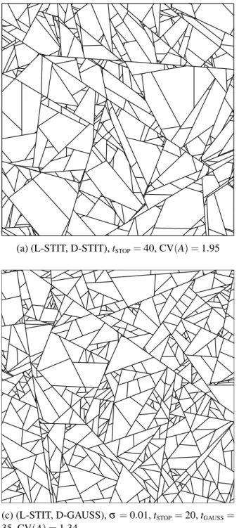
(a) (L-STIT, D-STIT),tSTOP=40, CV(A) =1.95 (b) (L-AREA, D-STIT),tSTOP=512, CV(A) =1.26

(c) (L-STIT, D-GAUSS),σ=0.01,tSTOP=20,tGAUSS= 35, CV(A) =1.34

(d) (L-AREA, D-GAUSS), σ = 0.01, tSTOP = 30, tGAUSS=450, CV(A) =0.82

Fig. 2: Simulations of isotropic tessellations with different lifetime distributions L and division rules D. In all the realizations are about 500 cells.

by the Miles-Lantuejoul method (Serra, 1982; Chiu

et al., 2013). Any cell which does not intersect the boundary of the window is given a weight, which is proportional to the reciprocal of the probability that this cell is completely contained in the window. This compensates for the different chances of the cells to appear completely inside the window. In a square window of side lengthaand parallel to the horizontal and vertical axes, the weight of a cellz⊂Wis

w(z) = 1

(a−b(z,0))(a−b(z,π/2)).

The formula to calculate the mean area of the cells in a given simulation is

MEAN(A) = 1

∑z⊂Ww(z)z

∑

⊂W

w(z)A(z),

(8)

MSE(A) = 1

∑z⊂Ww(z)z

∑

⊂W

w(z) (A(z)−MEAN(A))2,

the estimated standard deviation is SD(A) =

p

MSE(A),and the estimated coefficient of variation is CV(A) =SD(A)/MEAN(A).

For the other entities, the corresponding formulae are obtained by simply replacing the symbol Aby P,

RD,b_max,b_min,ASR, respectively.

The isoperimetric quotientRDand the aspect ratio

ASR are invariant with respect to scaling, and they provide information about the shapes of the cells. For all the entities the coefficient of variation CV is scale invariant and expresses the variability of these entities within a realization of the tessellation, i.e., a small value of CV means that the structure is more ’homogeneous’,i.e., the differences between the individual cells are relatively small. The CV is a useful and efficient criterion for checking the goodness-of-fit of a model to a real structure.

Fig. 2 shows realizations of isotropic tessellations for the STIT model and for the three modifications. In (a) and (b) the simulation was performed in a window of size 1. For D-GAUSS the window size for the simulation was 2, and then the central part of size 1 was cut out and this is shown in (c) and (d). The timestSTOP, andtGAUSS are chosen such that in all

cases there are about 500 cells. The very tiny cells are not visible in these panels. A comparison of the stopping times for L-STIT and L-AREA indicates that the division process is considerably slower when the lifetime distribution of the cells depends on the area.

COMPARISON OF THE MODELS –

A SIMULATION STUDY

Whereas there are numerous theoretical results for STIT tessellations, the modified models can (up to now) only be investigated by simulation studies. We have considered some examples in order to see how the modified models differ from STIT – and how they depend on the choice of their parameters.

Besides ISO and ELLIP, we focused on the directional distributions RECT and DRECT.

Some results of our simulation study are given in the Tables 1 and 2. The data are based on 100 repetitions of simulations with window side 1. The number of cells is indicated in order to show the sample sizes the estimated values are based on. Our focus is on the scale-independent CV-values, not on the number of cells. Clearly, the number of cells can

be increased by increasingtSTOPortGAUSS, respectively.

But there is no theoretical basis to control the number of cells in the modified tessellation models.

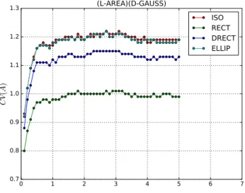
In Figs. 3 and 4, for D-GAUSS the estimated values of CV(A) are plotted againstσ, 0.1≤σ ≤5.

For the elliptic directional distribution the parameter is

bellip=0.1. The simulations for Fig. 3 are performed

with tSTOP = 32, tGAUSS = 256 and for Fig. 4 are

performed with tSTOP = 1024, tGAUSS = 2048. Each

value is based on 50 repeated simulations in a window of size 1.

0 1 2 3 4 5 6 7

σ

1.0 1.2 1.4 1.6 1.8 2.0

C

V(

A

)

(L-STIT)(D-GAUSS)

ISO RECT DRECT ELLIP

Fig. 3: The value of CV(A)as a function ofσ for

(L-STIT, D-GAUSS).

0 1 2 3 4 5 6 7

σ

0.7 0.8 0.9 1.0 1.1 1.2 1.3

C

V(

A

)

(L-AREA)(D-GAUSS)

ISO RECT DRECT ELLIP

Fig. 4: The value of CV(A)as a function ofσ for

(L-AREA, D-GAUSS).

We summarize our observations.

(9)

Table 1: Values of CV for D-STIT withtSTOP=32 for L-STIT andtSTOP=256 for L-AREA. In the cases DRECT

and ELLIP parameterbellip=0.05.

D-STIT L-STIT L-AREA

CV # cells CV # cells

ISO

Area 1.84±0.27

282±54

1.17±0.09

198±15 Isoper. Quotient 0.31±0.02 0.30±0.02

Max Width 0.85±0.06 0.63±0.04 Min Width 0.98±0.07 0.72±0.04 Aspect Ratio 0.42±0.02 0.41±0.02

RECT

Area 1.63±0.21

223±40

0.98±0.07

202±17 Isoper. Quotient 0.45±0.03 0.44±0.03

DRECT

Area 1.72±0.26

227±45

1.06±0.10

202±16 Isoper. Quotient 0.45±0.03 0.45±0.02

ELLIP

Area 1.48±0.22

77±18

1.15±0.09

167±15 Isoper. Quotient 0.57±0.05 0.57±0.04

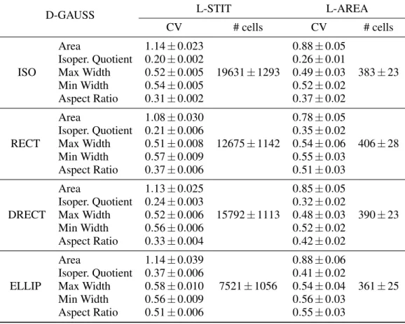
Table 2: Values of CV for D-GAUSS with σ =0.01 and tSTOP =32, tGAUSS =256 for L-STIT and tSTOP =

256,tGAUSS=512 for L-AREA. In the cases DRECT and ELLIP parameterbellip=0.1.

D-GAUSS L-STIT L-AREA

CV # cells CV # cells

ISO

Area 1.14±0.023

19631±1293

0.88±0.05

383±23 Isoper. Quotient 0.20±0.002 0.26±0.01

RECT

Area 1.08±0.030

12675±1142

0.78±0.05

406±28 Isoper. Quotient 0.21±0.006 0.35±0.02

DRECT

Area 1.13±0.025

15792±1113

0.85±0.05

390±23 Isoper. Quotient 0.24±0.003 0.32±0.02

ELLIP

Area 1.14±0.039

7521±1056

0.88±0.06

361±25 Isoper. Quotient 0.37±0.006 0.41±0.02

(10)

than for (L-STIT, D-STIT). This is not surprising, because for small values ofσ the lines tend to divide

the cells more ’central’, see also Fig. 2. The Fig. 3 and Fig. 4 illustrate the dependence on σ of CV(A). The apparent limit for increasingσis plausible because the

truncated Gauss distribution converges to the uniform distribution on the respective interval and thus the difference between D-GAUSS and D-STIT vanishes. It is remarkable, that even for very smallσ the CV(A)

is never smaller than 1. We checked this also for values

σ =10−4. This phenomenon is observed for all the

considered directional distributions. Obviously, CV(A)

also depends on the directional distribution, see Table 2. Notice, that in real crack patterns, as shown in the section below or in Nagel et al. (2008), CV(A) is clearly smaller than 1.

A reason for the apparently large lower bound for CV(A)is that the lifetime distribution L-STIT does not depend on the area of a cell z, but on Θ([z]), which

is for the directional distributions ISO and RECT proportional to the perimeter of z. This motivates an investigation of the AREA, D-STIT) and (L-AREA, D-GAUSS) models. And indeed, the CV(A) is distinctly smaller than in the corresponding L-STIT models.

We remark, that for the (L-AREA, D-STIT) model with the directional distribution RECT we have a theoretic result that CV(A) =1 asymptotically, when the window side goes to infinity (a manuscript in preparation by Mart´ınez and Nagel).

For (L-AREA, D-GAUSS), our simulations with

σ =0.01indicate, that for DRECT the CV(A) seems

not considerably depend on the parameter bellip, we

observed CV(A)≈0.7 for all 0.001≤bellip≤1.

Qualitatively, CV(bmax) and CV(bmin) behave

similar as CV(A), but quantitatively, the changes of the values are small.

In the cases which we considered, the CV of the isoperimetric quotientRDand of the aspect ratioASR

seems not to change significantly between L-STIT and L-AREA for the division rule D-STIT. But for the division rule D-GAUSS, the CV for L-AREA are larger than for L-STIT.

AN EXAMPLE OF EXPERIMENTAL

CRACKING

Sample preparation and microscopy: The experimental cracking shown in Fig. 5 was obtained by metallizing polydimethylsiloxane (PDMS).

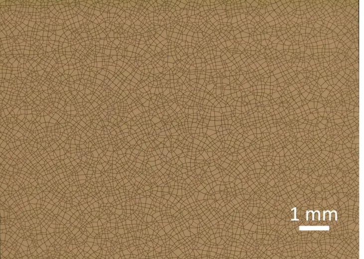
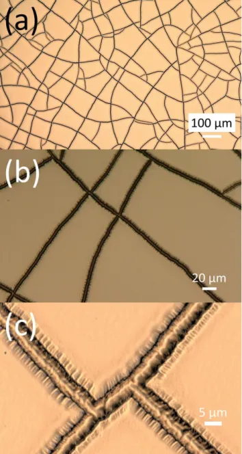
The details of the fabrication can be found in a previous article (Seghir and Arscott, 2015) published by one of the authors. In the case here, the specific metallization was a chromium/gold (20/100 nm) bilayer film deposited using thermal evaporation. Prior to metallization, the PDMS had been treated with an appropriately-dosed oxygen plasma to create a thin brittle silica film on the surface of the PDMS – this brittle film enables the observed “mud-cracking” seen in Fig. 5. The cracking is due to the process-induced stress present in the thermally-evaporated chromium film – which is known to be high. The gold regions in the figure are the uniform chromium/gold layer, the black lines are the cracks in the metallization and the brittle silica surface layer. The large field image shown (12×8.7 mm, 12 425×9 021 pixels of side length 0.96 µm) in the figure was produced using optical microscopy by stitching together 144 images using a digital microscope VHX-6000, Keyence, Japan. Fig. 6 shows zoom images of the cracking.

The result of image analysis is shown in Table 3. The area A(z) of the cells is estimated by pixel counting,i.e., ˆA(z) =nc2, wherenis the pixel number andcis the pixel size. The cells are convex, and hence the accuracy of ˆA(z) can be estimated based on the Steiner formula (Schneider and Weil, 2008). Let Br

denote the circle with radiusr, centered in the origin, and ⊕ the Minkowski subtraction and addition, respectively. From z Br ⊆z⊆z⊕Br it follows for

r=c/12 that

A(z)− c

12P(z)/Aˆ(z)/A(z) +

c

12P(z) +

πc2

144. Hence, the relative deviation δ(Aˆ) = (Aˆ(z) −

A(z))/A(z) from the true area A(z) can be estimated by

cP(z)

12A(z) /δ(Aˆ)/

12cP(z) +πc2

144A(z) .

This formula shows the influence of the lateral resolution, expressed bycon the error bounds. If,e.g.,

c=1 µm andzis a square of the side length 20 µm, the above estimate yields−1.667 %/δ(Aˆ)/1.672 %.

The estimation of the perimeter P(z) is usually based on a discrete version of one of Crofton’s intersection formulae (Ohser et al., 1998), where the discretization is induced by the sampling of the continuous setzon a square point lattice of spacingc. Let ˆP(z) be an estimate of the perimeter and δ(Pˆ) =

ˆ

P(z)−P(z)/P(z). Then the Steiner formula and same arguments as for the area yield

− πc

12P(z) /δ(Pˆ)/

πc

12P(z),

(11)

Fig. 5: Optical microscopy image of cracking of metallized (Cr/Au – 20/100 nm) PDMS. The metallization is indicated in gold, the cracks in black where the PDMS is visible. The metallization is a chromium/gold bilayer having a thickness of 20/100 nm. The image was taken using a digital optical microscopy VHX-6000, Keyence, Japan. The image (12×8.7 mm, 12 425×9 021 pixels of side length 0.96 µm) is composed of 144 images stitched together.

The minimal and the maximal widths are estimated using the convex hull C of the set of pixels belonging to z, where in our approach the convex hull was effectively determined using Graham’s scan algorithm (Graham, 1972). The estimates are ˆbmin(z) =

b_min(C) +c and ˆbmax(z) =bmax(C) +c, respectively.

Thus, the relative errors of these estimators should be between−c/12 andc/12.

As the isoperimetric quotient and the aspect ratio are ratios of random numbers, it is difficult to estimate their errors. However, it is expected that also for these ratios the errors decrease with decreasing pixel sizec.

Nevertheless, for very small cells the relative error can be large. In our example, Fig. 5 consists of 12 425×9 021 pixels of side length 0.96 µm. Therefore, we believe that we have found a good balance of sufficiently high lateral resolution and sufficiently large sample size, as a basis for reasonable statistics.

Let us consider the sample of a crack pattern shown in Fig. 5 and check whether one of the presented models can approximately be fitted. At a first glance, one does not see preferred directions, and thus the overall directional distribution can be isotropic. But comparing the sample with the simulations for the directional distribution ISO, it becomes obvious that ISO will not be appropriate. In particular, in the sample the proportion of quadrangles is considerably higher than in the models with ISO. Therefore, we choose a disturbed discrete directional distribution DRECT with the parameter 0<b_ellip<1.

(12)

Fig. 6: Zoom images of the cracking taken using the optical microscope. (a) ×200 magnification/pixel size = 1.06 µm, (b) ×1000 magnification/pixel size = 0.2 µm, and (c) ×5000 magnification/pixel size = 0.044 µm. In (c) the crack width is 5.45±0.34 µm.

As a first goodness-of-fit criterion we consider CV(A), the coefficient of variation of the cell areas. It is a scale invariant statistic, and it is rather robust concerning digitization effects in image analysis.

As shown in Table 4, the choice bellip = 0.1,

σ =0.1, tSTOP = 500, tGAUSS =2 000, window side

a =1, yields a good approximation for CV(A). An obvious flaw is that the shape indicators MEAN(RD)

and MEAN(ASR) are too small compared to the data in Table 3. Regarding an example of a tessellation

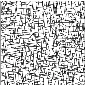
as shown in Fig. 7, one can see that there appear numerous acute triangles which we do not observe in the sample in Fig. 5, and such triangles have small values of RD and of ASR. It will be a subject of our future work to modify the model by suppressing small angles between the edges of the tessellations. Regarding the scale dependent entities, for the mean area and the mean perimeter, 1 unit of the simulation scheme corresponds to 894 µm and 750 µm, respectively. For Min Width the scaling factor is about 1000, and for Max Width it is about 700 which emphasizes the weak adaption of the model concerning the shape indicators.

Table 3: Statistical data for Fig. 5.

MEAN SD CV

Area (µm2) 403.515 319.725 0.794 Perimeter (µm) 75.075 31.185 0.415 Isoper. Quotient 0.787 0.109 0.138 Min Width (µm) 18.375 8.295 0.451 Max Width (µm) 28.56 11.445 0.401 Aspect Ratio 0.644 0.127 0.198

Table 4: Statistical data for simulated tessellations (50 replications) for (L-AREA, D-GAUSS), DRECT,

bellip = 0.1, σ = 0.1, tSTOP = 500, tGAUSS = 2 000,

window sidea=1.

MEAN SD CV

Area 0.0005 0.0004 0.7896 Perimeter 0.0998 0.0423 0.4235 Isoper. Quotient 0.5759 0.1682 0.2921 Min Width 0.0168 0.0079 0.4688 Max Width 0.0411 0.0191 0.4648 Aspect Ratio 0.4385 0.1689 0.3853

DISCUSSION

(13)

Fig. 7: Example of a simulated tessellation with (L-AREA, D-GAUSS), DRECT, b_ellip =0.1, σ = 0.1,

tSTOP=500,tGAUSS=2 000, window sidea=1.

The new models enable good results concerning the important statistical parameter CV(A), the coefficient of variance of the cell areas. On the other hand, there are several obvious features of real crack patterns which are not yet understood, e.g., in many crack patterns, a dividing line tends to meet at right angles with the boundary of the cell, rather than at small angles. This motivates future work aimed at feasible parametric models which allow for a reasonably good approximation of actual crack patterns.

ACKNOWLEDGMENT

Werner Nagel was repeatedly supported by the Centro de Modelamiento Matem´atico (CMM) de la Universidad de Chile, Project Basal AFB170001 Conicyt.

The work of Steve Arscott was in part funded by the French ‘RENATECH’ network. The digital microscope was purchased within the French ANR funded project ‘TIPTOP 1’ (ANR-16-CE09-0029).

Mat´ıas Vargas from Facultad de Ingenier´ıa de la Universidad Andr´es Bello worked on the development of the simulation program web page.

The authors thank the referee and the editor for their helpful comments.

REFERENCES

Boulogne F, Giorgiutti-Dauphin´e F, Pauchard L (2015). Surface patterns in drying films of silica colloidal dispersions. Soft Matter 11:102–8.

Chiu SN, Stoyan D, Kendall WS, Mecke J (2013). Stochastic geometry and its applications, 3rd Ed. Chichester: John Wiley & Sons.

Cowan R (2010). New classes of random tessellations arising from iterative division of cells. Adv Appl Probab 42:26–47.

Graham RL (1972). An efficient algorithm for determining the convex hull of a finite planar set. Inform Process Lett 1:132–3.

Hafver A, Jettestuen E, Kobchenko M, Dysthe DK, Meakin P, Malthe-Sørenssen A (2014). Classification of fracture patterns by heterogeneity and topology. EPL Europhys Lett 105:56004.

Hutchinson J, Suo Z (1991). Mixed mode cracking in layered materials. Adv Appl Mech 29:63–191.

Iben HN, O’Brien JF (2006). Generating surface crack patterns. Graph Models 71:198–208.

Kumar A, Pujar R, Gupta N, Tarafdar S, G.U. K (2017). Stress modulation in desiccating crack networks for producing effective templates for patterning metal network based transparent conductors. Appl Phys Lett 111:013502.

Le´on R (2019). Crack pattern simulation. http: //crackpatternsimulation.informatica-unab-vm.cl/. Mecke J, Nagel W, Weiß V (2008). A global construction

of homogeneous random planar tessellations that are stable under iteration. Stochastics 80:51–67.

Mosser L, Matth¨ai S (2014). Tessellations stable under iteration. Evaluation of application as an improved stochastic discrete fracture modeling algorithm. In: Proc 2014 Int Discrete Fracture Network Eng Conf 163–76. Nagel W, Mecke J, Ohser J, Weiß V (2008). A tessellation

model for crack patterns on surfaces. Image Anal Stereol 27:73–8.

Nagel W, Weiß V (2005). Crack tessellations: characterization of stationary random tessellations stable with respect to iteration. Adv Appl Probab 37:859–83.

Nandakishore P, Goehring L (2016). Crack patterns over uneven substrates. Soft Matter 12:2253–63.

Ohser J, Schladitz K (2009). 3D images of materials structures – Processing and analysis. Weinheim, Berlin: Wiley VCH.

Ohser J, Steinbach B, Lang C (1998). Efficient texture analysis of binary images. J Microsc 192:20–8. Schneider R, Weil W (2008). Stochastic and integral

(14)

Seghir R, Arscott S (2015). Controlled mud-crack patterning and self-organized cracking of polydimethylsiloxane elastomer surfaces. Sci Rep 5:14787–802.

Serra J (1982). Image analysis and mathematical morphology. London: Academic Press.

Stoyan D, Mecke J, Pohlmann S (1980). Formulas for stationary planar fibre processes. II. Partially oriented fibre systems. Math Operationsforsch Statist Ser Statist 11:281–6.

Thouless M, Evans A, Ashby M, Hutchinson J (1987). The edge cracking and spalling of brittle plates. Acta Metall Mater 35:1333–41.

Xia Z, Hutchinson J (2000). Crack patterns in thin films. J Mech Phys Solids 48:1107–31.