ADAPTIVE CROSSING NUMBERS AND THEIR APPLICATION TO
BINARY DOWNSAMPLING
ETIENNE
DECENCIÈRE AND
MICHEL
BILODEAU
Centre de Morphologie Mathématique, Ecole des Mines de Paris, 35, rue Saint Honoré, 77305 Fontainebleau CEDEX, France
e-mail: [email protected]
(Accepted May 21, 2007)
ABSTRACT
A downsampling method for binary images is presented, which aims at preserving the topology of the image. It uses a general reference sampling structure. The reference image is computed through the analysis of the connected components of the neighbourhood of each pixel. The resulting downsampling operator is auto-dual, which ensures that white and black structures are treated in the same way. Experiments show, by visual inspection on the displayed images, that the image topology is indeed preserved satisfactorily.
Keywords: binary downsampling, digital topology, reference downsampling.
INTRODUCTION
In this era of expanding mobile multimedia devices, small screens will soon be in every pocket. Their relatively small resolutions (the screen of a Personal Digital Assistant (PDA) is typically 320 by 320 pixels) pose display problems, worsened by the fact that visual digital documents are often thought for high resolution displays. For example, how can a faxed document, or a tourist brochure, scanned with a 200 dpi resolution, be conveniently displayed on a PDA screen?
As it can be seen, we are confronted with a severe downsampling problem. Moreover, these images often are binary or nearly so, like faxes, diagrams, maps, etc. In these particular cases, classical downsampling methods work very badly, because they aim at removing from the image those structures which cannot be represented at a lower resolution level. For example, depict a thin black line on a white background. If downsampled with a classical linear method (i.e., high frequencies are filtered out before downsampling), this line will be smoothed away. If we require that the resulting image is binary, thin structures might be simply erased. In many application domains this is a normal, and welcome, feature. However, when displaying graphical data on small displays, the opposite might be more interesting, that is, preserving small structures when there is enough place in the image. In the case of binary images, this constraint can be expressed in mathematical terms as a homotopy preservation property.
This application was the initial motivation for our work, which explains some of the choices made during the study. However, very similar problems can be
found in other application domains. The following ones can be cited:
– multi-resolution representation of binary shapes for pattern recognition, a problem which has been studied by Borgeforset al.(1996; 1999; 2001);
– multi-resolution display of labelled images. After this introduction, we will define the framework, and review the existing methods. Then, in section “Reference downsampling”, we will introduce a general adaptive downsampling scheme which will be used as basis in the following section for a binary downsampling method which aims at preserving homotopy. In the next section the results are presented and commented. Finally, conclusions are drawn.
Note that a first, shorter version of this paper was presented in the International Symposium for Mathematical Morphology (Decencière and Bilodeau, 2005).
FRAMEWORK AND OBJECTIVES
Only binary 2D images will be considered in this paper. They typically correspond to text, diagrams, graphics, or maps.
Of course, the detection of what is important is not trivial, nor it is easy to know how long it is possible to preserve data which is considered meaningful along several downsampling steps. We have made the hypothesis that the image topology is closely related to the correct perception of the binary image. Therefore, our goal is to produce a downsampling operator that preserves the image topology, when possible. Indeed, it is evident that in many cases, when resolution decreases, the resulting downsampled image cannot be homotopic to the original image. For example, a checkerboard image, where each pixel corresponds to one square, cannot be downsampled homotopically. However, in many other cases we believe that a topological approach might give interesting results.
When analysing binary images from a topological point of view, to avoid problems that will be seen latter, in practice one often treats differently the “object” pixels and the “background” pixels. In our framework, we do not know beforehand if the important structures of a binary image are black or white. Therefore, we will treat them in the same way. In other words, the downsampling method should be auto-dual. Another reason for the adoption of this hypothesis is our wish to extend these results to gray scale images, where making a difference between “objects” and “background” is often impossible.
STATE OF THE ART
The classical linear downsampling approach is based on the removal from the original image of those frequencies which are too high to be represented at a lower resolution level. They can be adapted to our framework by applying a convenient threshold after downsampling, in order to recover a binary image. The resulting downsampling operator can be auto-dual, however, preserving topological properties this way is not straightforward, as it will be shown in section “Results”.
Morphological downsampling methods are also based on the same idea (Haralick et al., 1989; Heijmans and Toet, 1991; Florêncio and Schafer, 1994): first, they remove those structures which are considered too small to be represented at a lower resolution level, and then a point downsampling is applied. Clearly, this kind of approach is not adapted to our application.
In a series of articles, Borgeforset al.(1996; 1999; 2001) propose a multiscale representation of binary images. Their aim is to preserve the shape of the objects. Even if these methods tend to preserve the topology of the image, this is not their main objective.
Furthermore, the proposed downsampling methods are not auto-dual, an essential property in our framework.
Adaptive downsampling methods analyse the image contents before downsampling in order to preserve meaningful details when possible. A method based on the morphological tophat transformation has been proposed for downsampling grey level and binary images (Decencière et al., 2000; 2001). It takes into account the size of the structures, by comparison with a structuring element (i.e., a reference set), in order to favour those pixels which are considered more interesting. In this paper, we will adapt this approach to the case of binary images but, instead of geometric information, topological information will be used.
REFERENCE DOWNSAMPLING
A general reference downsampling method has been introduced by Decencièreet al.(2000; 2001). We present below a version adapted to binary images.
A binary imageIis a binary function ofZ2:
I: Z2 −→ {0,1}
(x,y) 7−→ I(x,y).
The set of binary images is denoted I. In the
following, animagewill mean abinary image. We will often identify an imageIto the set{p∈Z2|I(p) =1}.
For instance, when we say that a point m of Z2 belongs toI, we mean:m∈ {p∈Z2 |I(p) =1}. The inverse image ofI is ¯I=1−I. A point of Z2 is also called a pixel. We will use the letters p,q,m or their coordinates (x,y) to denote them. We will adopt the
usual convention to represent binary images: pixels where the image is equal to 1 will be represented in black, whereas the others will be represented in white. Let us partitionZ2 into 2×2 blocks. For all(x,y)
inZ2:
B(x,y) ={(2x,2y),(2x+1,2y),
(2x,2y+1),(2x+1,2y+1)}. (1)
This partition is the base for the construction of the downsampling operator.
Definition 1 (Binary downsampling operator) A binary downsampling operator ∆ is a function from I intoI such that, for every I∈I and(x,y)∈Z2:
(∆(I))(x,y)∈ {I(2x,2y),I(2x+1,2y),
Therefore, the main question when defining a binary downsampling operator will be how to choose the value of(∆(I))(x,y)among the setI(B(x,y)).
A grey level image R is a function of Z2 into
{0, . . . ,255}:
R: Z2 −→ {0, . . . ,255}
(x,y) 7−→ R(x,y).
We define index_max(R,B(x,y)) as the element
of B(x,y) where R takes its maximal value. If there
were two or more elements ofB(x,y)whereRtook its
maximal value, then the first of these in video scanning order would be taken.
Definition 2 (Reference downsampling operator)
Let R be a grey level image. The binary downsampling operator∆Rwith reference R is defined as:
∆R: I −→ I
I 7−→ ∆R(I) =I(index_max(R,B(.)).
The simplest binary downsampling method, called point sampling, which consists in taking the first pixel of eachB(x,y), is equivalent to applying a reference
downsampling operator with a constant reference image. Needless to say, this method gives very poor results.
The choice of R is essential to build interesting sampling operators. The objective of this approach is to buildRfromI, in such a way that the value ofR(x,y)
corresponds to the importance we want to give to pixel
(x,y)in imageI.
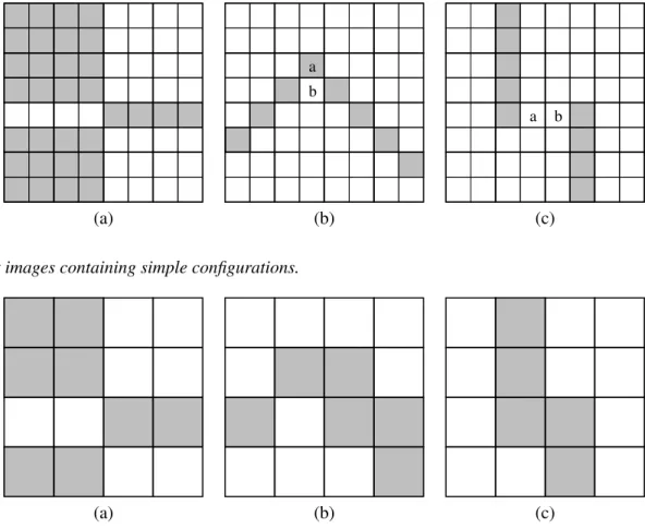
Fig. 1a shows an image to illustrate our purpose. First of all, note that point sampling would produce a completely white image. Methods which favour “black” pixels (pixels belonging to the image) would produce image in Fig. 1b. This would be the case for instance if we used the same initial image as reference image in the binary downsampling operator. The result is considerably better than the result obtained with point sampling, but there has been a topological modification of the image (it will be seen in the next section what is exactly meant by this). Such modifications are often annoying when dealing with binary data. For example, in this case, image (a) would be interpreted as a letter “C”, whereas image (b) would be misunderstood as a letter “O”. We would like to compute a reference image that would give the result shown by image (c) through reference downsampling. To achieve this, pixel c in the first image should be considered more important than pixelsaandb, which means that the corresponding value in the reference
image should be larger than the values associated to the other two pixels.
In the next section we will propose a method to build a reference image wich takes into account the image topology.
BUILDING A REFERENCE IMAGE
DIGITAL TOPOLOGY: A DUAL FRAMEWORK
We recall the main digital topology notions that will be used in the following. For a complete introduction to digital topology, the reader may consult the article by Kong and Rosenfeld (1989).
LetN be a neighbourhood relation onZ2,i.e., a
binary relation onZ2which is symmetric. When points
pandmofZ2are in relation throughN, we say that
they are neighbours and we writepN m. Moreover, we
adopt the following convention: we takeN such that
a point p is never in relation with itself through N .
We will denote N(p) the set of neighbours of p. As pN pis always false, pnever belongs toN(p).
Two subsetsAandBofZ2 will be said to beN
-neighbours if they are disjoint and there are two pixels
m and p respectively belonging to A andB such that
pNm.
Once equipped with a neighbourhood relation, the points of an image can be aggregated into larger structures.
A sequence (q0, . . . ,qK) of points of Z2, where
K is a strictly positive integer, is a N -path if and
only if any two consecutive points of the sequence are
N -neighbours. The pixels q0 and qK are called the
extremities of the path.
Two different points m and p belonging to an image I are said to be N-connected in I if there is
a path included inIwhose extremities aremandq. “To be connected in I” is an equivalence relation. Its equivalence classes are theN -connected
components ofI. The number, possibly infinite, ofN
-connected components of a subset ofZ2or an imageI will be denotedCCN(I).
We now introduce the notions of interior and isolated point, in a general form adapted to our framework. A point pofZ2is said to be aN -interior pointofI if and only if each of itsN-neighbours has
a c b
(a) (b) (c)
Fig. 1.(a) Example of binary image. (b) Downsampled image when favoring black pixels. (c) Aimed result.
Typical neighbour relations used in image processing are the 4-, 6- and 8- neighbourhoods, respectively denoted N4, N8 and N6. Among these, N6 has the best topological properties, as it is the
only one that fulfills the digital Jordan curve theorem. But when the image has been digitized following a square grid, 6-neighbourhood causes some unwelcome phenomena. The Khalimsky neighbourhood relation, denotedNK, should also be mentioned. It shows very
nice topological characteristics, but it is not translation invariant: if both coordinates of a pixel pare even or uneven, thenNK(p) =N8(p). For all other pixels, we
haveNK(p) =N4(p).
In order to palliate the defects of 4- and 8- neighbourhoods, neighbourhood relations which depend on the image have been proposed, and widely used. For example, the (8,4)- neighbourhood relation
N8I
,4is defined as:
pN8I
,4m ⇔
½
pN8m if I(p) =1 and I(m) =1 pN4m otherwise.
(2) The (4,8)- neighbourhood relation,N4I
,8, is defined
analogously. We make explicit the dependance of the neighbourhood on the image by puting I
as a superscript on N. These image-dependent
neighbourhoods fulfill the digital Jordan curve theorem (see Kong and Rosenfeld, 1989, for references to the various demonstrations).
The N -homotopy graph of an image can now
be introduced. Note that very similar notions are called “adjacency tree” in Kong and Rosenfeld (1989), “homotopy tree” in Serra (1982) and “adjacency graph” in Kong and Roscoe (1985).
Definition 3 (N -homotopy graph) Let I be an image and N a neighbourhood relation. The N -homotopy graph of I is the non-directed graph whose
vertices are the N -connected components of I and
¯
I, and whose edges link N -neighbouring connected components. If V is the set of its vertices, and E the set of its edges, then the graph will be simply denoted (V,E).
When the neighbourhood relation N is in fact N8I
,4 orN4I,8, the homotopy graph is a tree (see Kong
and Rosenfeld, 1989, and references within).
Note that this definition is slightly different from the ones given in Kong and Rosenfeld (1989) and Serra (1982). Indeed, no supposition is made about the color of the background. This allows “black” and “white”pixels to play symmetric roles. In fact, ifN is
inversion invariant, thenI and ¯I will have isomorphic graphs, and therefore will be considered homotopic in this framework.
Definition 4 (N -homotopic images) Let N be a neighbourhood relation. Two images are N -homotopic if and only if their corresponding N -homotopy graphs(V1,E1)and(V2,E2)are isomorphic,
i.e., if and only if there is a bijection f between V1and V2such that(A,A0)∈E1if and only if(f(A),f(A0))∈
E2.
“To beN-homotopic” is an equivalence relation.
Its equivalence classes are theN-homotopy classes of I.
Let us consider an image I and a pixel p. Let J
be the image equal toI on all pixels ofZ2 except on
p. When p belongs to I, the construction of J is the essential basic step to compute a thinning operator. For the thinning to be interesting, J and I must be homotopic. If this is true, then pis said to be asimple point. More generally, in our dual framework:
Definition 5 (N-simple point) A point ofZ2 is N -simple with respect to a given image if and only if the inversion of its value does not modify theN-homotopy class of the image.
As in image thinning, simple points will play an important role in image downsampling. Indeed, it is important to note that, if the modification of a single simple point does not modify the topology of the considered image, the simultaneous modification of two simple points might do so. This problem, found in image thinning, will appear in our study: the simultaneous disappearance of two simple points through the downsampling procedure might introduce topological modifications.
In 2D, simple points can be simply characterized by the study of their neighbourhood.
ADAPTIVE CROSSING NUMBERS
The study of the number of connected components of N(p)∩I has lead to several notions, namely
the Rutovitz crossing number (Rutovitz, 1966), the Hilditch crossing number (Hilditch, 1969), and the Yokoi connectivity number (Yokoiet al., 1973).
However, these crossing numbers are only defined for pixels belonging to the image. We will now introduce an image inversion invariant crossing number.
In order to define adaptive crossing numbers, we first have to classify the pixels of the image as object pixels or background pixels. Note that we will call object pixels those pixels that are considered important because they belong to the minority in their neighbourhood; they might be black or white. We will then consider an 8-neighbourhood for object pixels, and a 4- neighbourhood for the other pixels.
Consider a pixelpand a binary imageI. In order to answer the question “doespbelong to the object”, we compute the numbernI(p)of 8-neighbours ofpwhere Itakes the same value as on p. This is given by:
nI(p) =Card({q∈N
8(p) |I(q) =I(p)}), (3)
whose values are included between 0 (N8-isolated
point) and 8 (N8-interior point). If this value is equal or
greater than 4, then we will considerpas a background pixel, otherwise, as an object point.
Proposition 6 The operator nI is invariant with respect to image inversion:
∀I∈I,∀p∈Z2,nI(p) =nI¯(p). (4)
Demonstration
nI(p) =Card({q∈N8(p) |I(q) =I(p)})
=Card({q∈N8(p) |I¯(q) =I¯(p)}) =nI¯(p)
¤
An immediate consequence of this proposition is that the notion of object pixel is inversion invariant.
Let us consider a pixelp. It is either an object pixel ofI, or a background pixel ofI.
If p is an object pixel of I (i.e., nI(p)<4), then
we consider its 8-neighbours (see Fig. 2a). On some of these neighbours, I takes a different value from p; we call the number of N4-connected components of
this subset theadaptive crossing numberof the object pixelp.
Similarly, if p is a background pixel of I (i.e.,
nI(p) ≥4), then we consider its 4-neighbours (see
Fig. 2b). On some of these neighbours, I takes a different value from p; we call the number of N8
-connected components of this subset the adaptive crossing numberof the background pixelp.
For example, in Fig. 2a, the number of 4-connected components of the set{m∈N8(a)|I(m)6=I(a)}is 1,
and in Fig. 2b, the number of 8-connected components of the set{m∈N4(c) |I(m)6=I(c)}is 2.
More formally:
Definition 7 (Adaptive crossing number) The adaptive crossing number of a pixel p in an image I, denoted XI(p), is:
XI(p) =
CCN4({m∈N8(p)| I(m)6=I(p)}, if nI(p)<4, CCN8({m∈N4(p)| I(m)6=I(p)},
if nI(p)≥4,
(5)
where CCN(I) is the number of N-connected components of a subset ofZ2or an image I.
a
c
2 1 3 2 2
2 2 2
1 1 1 1 1
1 1 2 2 1
0 c a
1 2 1 b
(a) (b) (c)
Fig. 2.(a) Pixels around pixel a considered to compute its adaptive crossing number. Neighbourhood relation on them, used to compute XI(a), indicated by segments. (b) Pixels around pixel c considered to compute its adaptive crossing number. Neighbourhood relation on them, used to compute XI(c), indicated by segments. (c) Test image with some values of the adaptive crossing number. Notice that the value associated to pixel c is higher than those given to a and b.
Proposition 8 XI is invariant with respect to image inversion:
∀I∈I,∀p∈Z2,XI(p) =XI¯(p). (6)
Demonstration Simply rewrite equation 5 using proposition 6.¤
Note that an adaptive neighbourhood relation could be defined in exactly the same way: 8-neighbourhood would be considered between object pixels, and 4-neighbourhood otherwise. However, this neighbourhood relation does not fulfill the Jordan curve theorem.
As a consequence, the reference image RI n built
from XI is also invariant with respect to image
inversion:
RIn(p) =
½
XI(p) if XI(p)>0,
5 otherwise. (7)
The particular case forXI(p) =0,i.e., for isolated
points, is necessary if we want these pixels to be preserved. The value 5 is arbitrary; it has to be higher than the other values ofXI(p).
Finally, we obtain the following downsampling operator, that we call adaptive downsampling operator:
∆n(I) =∆RI
n(I), (8)
which has the property we were seeking for:
Theorem 9 The adaptive downsampling operator∆n is auto-dual:
∀I∈I,∆n(I) =∆n(I¯). (9)
Demonstration We have ∆n(I¯) = ∆RnI¯(I¯) and RIn = RI¯
n, therefore, for all(x,y)inZ2:
(∆n(I¯))(x,y) =I¯(index_max(RIn,B(x,y))
=1−I(index_max(RIn,B(x,y))
=∆RIn(I)
=∆n(I).
¤
RESULTS
First of all, in Fig. 2c we give the values ofXI(p)
for some pixels of the test image. Notice that the value associated to pixelc is now higher than the values of its neighbours a and b. Thanks to this, the resulting downsampled image with the reference imageRn we
have just defined is the one given by Fig. 1c.
Fig. 3 shows some more examples of simple configurations whose topology we would like to preserve.
Fig. 4 gives the result of the adaptive downsampling of the test configurations given in Fig. 3. As it can be seen, in the first case (Fig. 4a), the result is satisfactory. The images before and after downsampling are N -homotopic for all usual
neighbourhood relations N (including 4, 6, and
8 neighbourhoods, as well as (4,8) and (8,4)
a b
a b
(a) (b) (c)
Fig. 3.Test images containing simple configurations.
(a) (b) (c)
Fig. 4.Adaptive downsampling of test configurations.
auto-dual nature of the adaptive downsampling operator.
The second case (Fig. 4b) is slightly less satisfactory. The images before and after downsampling are for instance (8,4)-homotopic, but
not(4,8)-homotopic.
However, the third case (Fig. 4c) has not been conveniently downsampled. It is possible to build a reference image that would have preserved topology, but our method did not allow it. This problem is analogous to the problem of simple points during thinning operations. Indeed, pixels marked a and b
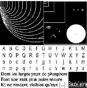
in Fig. 3c have an adaptive crossing number of 1. But, taken together, they are important to preserve the image topology. Their corresponding value in the adaptive reference image should be higher than the corresponding values of the neighbouring black pixels. Fig. 5 shows a more complex test image, containing geometric structures and text. Its size is 512×512. Fig. 6 shows the result of the application of the adaptive downsampling procedure.
Notice that adaptive downsampling has done a nice work in preserving some important structures. For example, in many cases topological downsampling
has avoided the fusion between letters. However, the proposed downsampling operator has not preserved some geometric details that are also important (look for instance at letters “t”, “j” or “r”). This is not surprising, given that the proposed downsampling operator only aims at preserving topology.
In some other cases (see for example letter “V” in Fig.6b) the topology of some structures has not been preserved. The main reason for this behavior is the lack of space (pixels per letter) in the resulting image. In some other cases, the local analysis does not correctly evaluate the value of some pixels (letters “h” or “y” in Fig.6b).
Finally, it should be noted that given that thin structures tend to be preserved along the downsampling process, their relative size will increase with respect to the larger structures.
In order to compare with state of the art downsampling methods, we have computed a gaussian pyramid from the initial image, see Witkin (1983).
(a) (b)
Fig. 6. (a) Adaptive downsampling. (b) Adaptive downsampling, iterated.
(a) (b)
The original image is first filtered using à 5×
5 support gaussian, and then point-sampled; the procedure is iterated to obtain the desired number of resolution levels. The resulting images are grey-level (values range between 0 and 255). In order to binarize them, we have used a threshold value of 127.5,
which gives a binary downsamplig operator which is also auto-dual. Fig. 7 shows the first downsampling step obtained this way. On top (a), the downsampled filtered image is shown, before thresholding. Note that it is a grey-level image, and that it is visually pleasing. However, the threshold (b) produces a much less pleasing result if compared with Fig. 6a. Thin structures have been erased.
CONCLUSION AND FUTURE
DEVELOPMENTS
As far as we know, the binary downsampling method we have presented is the first that uses purely topological criteria in the process.
It does a good job of preserving structures from a topology point of view, but, in some cases, the removal of two neighbouring simple points introduces topological modifications which could have been avoided. Therefore, a more subtle analysis is needed to compute a better reference image. For example, second neighbours could be considered in the analysis.
Moreover, it appears that a topology preservation criterion is not enough to preserve meaningful details. Some geometric information should be added to the reference image, as curvature or information about extremities. The reference downsampling approach allows to combine different sorts of information.
It should be noted that the operations involved in the computation of the reference image are not computationally greedy. The implementation of this method on mobile processors should not be a problem. The next step in this work will be to extend this downsampling approach to grey level images.
ACKNOWLEDGMENTS
This work has been financed by the European MEDEA+ Pocket Multimedia project.
REFERENCES
Borgefors G, Ramella G, Sanniti di Baja G (1996). Multiresolution representation of shape in binary images. In: Miguet S, Montanvert A, Ubéda S, eds. Discrete Geometry for Computer Imagery, Proceedings
DCGI’96, vol. 1176 of Lecture Notes in Computer Science. Lyon, France: Springer.
Borgefors G, Ramella G, Sanniti di Baja G (2001). Shape and topology preserving multi-valued image pyramids for multi-resolution skeletonization. Pattern Recogn Lett 22:741–51.
Borgefors G, Ramella G, Sanniti di Baja G, Svensson S (1999). On the multiscale representation of 2D and 3D shapes. Graph Model Im Proc 61:44–62.
Decencière E, Bilodeau M (2005). Downsampling of binary images using adpative crossing numbers. In: Ronse C, Najman L, Decencière E, eds., Mathematical morphology: 40 years on. Proceedings ISMM’2005. Paris, France.
Decencière E, Marcotegui B, Meyer F (2000). Content dependent image sampling using mathematical morphology. In: Goutsias J, Vincent L, Bloomberg D, eds., Mathematical Morphology and its applications to signal processing. Proceedings ISMM’2000. Palo Alto, CA, United States: Kluwer Academic Publishers. Decencière E, Marcotegui B, Meyer F (2001).
Content-dependent image sampling using mathematical morphology: application to texture mapping. Signal Process-Image 16:567–84.
Florêncio D, Schafer R (1994). Critical morphological sampling and its applications to image coding. In: Mathematical Morphology and its Applications to Image Processing. Proceedings ISMM’94.
Haralick R, Zhuang X, Lin C, Lee J (1989). The digital morphological sampling theorem. IEEE Trans Acoust Speech 37:2067–90.
Heijmans H, Toet A (1991). Morphological sampling. CVGIP—Image Understanting 54:384–400.
Hilditch C (1969). Linear skeletons from square cupboards. In: Meltzer B, Michie D, eds. Machine Intelligence, Vol. 4. Edinburgh: Edinburgh Univ. Press, 403–20.
Kong T, Roscoe A (1985). A theory of binary digital pictures. Comput Vision Graph 32:221–43.
Kong T, Rosenfeld A (1989). Digital topology: introduction and survey. Comput Vision Graph 48:357–93.
Rutovitz D (1966). Pattern recognition. J Royal Statist Soc 129:504–30.
Serra J (1982). Image Analysis and Mathematical Morphology—Volume I. New York: Academic Press. Witkin AP (1983). Scale-space filtering. In: Proceedings
of the 7th International Joint Conference on Artificial Intelligence.