Dynamical Simulation Models for the Development Process of Open Source Software Projects

Process of Open Source Software Projects

I. P. Antoniades, I. Stamelos, L. Angelis and G.L. Bleris Department of Informatics, Aristotle University

54124 Thessaloniki, Greece

Email: [email protected]

Abstract. There have been a few studies attempting to define the Open-Source software (OSS) development process in general terms and there have also been a few case studies of OSS projects. The latter studies presented qualitative and quantitative data for the OSS development process, managerial issues and pro-grammer attitudes. The authors in many cases offer descriptive explanations based on plausible assumptions but, as there is no general model to quantify their claims together with their possibly complicated interactions, the validity of such explanations cannot be directly demonstrated. Therefore, there is a need to move from descriptive models based on special cases to a more general

quantitative mathematical model that would hopefully reproduce real case re-sults. In the present paper we present a general framework for dynamical simu-lation models of the development process of OSS projects. Then we present a specific simulation model, which is demonstrated against results from available literature case study of the Apache OSS project. OSS dynamic simulation mod-els could serve as generic predicting tools of key OSS project factors such as project failure/success as well as time dependent factors such as the evolution of source code, defect density, number of programmers and distribution of work effort to distinct project modules and tasks.

1

Introduction

In Open Source Software development process work is not assigned; people under-take the work they wish to underunder-take, there is no explicit system-level design, no well-defined project plan, schedule or list of deliverables. A central management core group (which may also set certain code quality standards or rules) may screen code that is checked, but this process is much less strict than in closed source projects. Despite loose management and the chaotic nature of project evolution, the Open-source method has managed to produce some impressive products such as the Linux operating system, the Apache Web Server and the Perl language. Netscape has also launched an open-source project for Mozilla, its new Web Browser, proving that open-source is a serious candidate for the development of industrial software. Several other projects are used widely (such as SendMail, GCC) whereas there are more than 15,000 different OSS projects going on as of February 2, 2001, as shown by the SourceForge database (a free service supporting OSS projects - http://sourceforge.net) with more than 115,000 registered users.

There have been a few studies attempting to define the OSS development process in general terms [1-6] and there have also been a few case studies of OSS projects: Linux [7], Apache [8], FreeBSD[9], GNOME [10]. The latter studies presented some interesting qualitative data for the OSS development process, managerial issues and programmer attitudes as well as quantitative data regarding the total Lines of Code (LOC) added as a function of time, the defect density of the code produced, number of programmers and contributions per project module/task, average work-effort/time to submit a contribution (code change, defect correction, code testing) as well as other statistical measures. Despite the fact that these studies have produced interesting results validating or disproving certain hypotheses regarding OSS development on a per case basis, there is no sufficient global understanding, nor a precise definition of the open source development process: the results show both similarities as well as clear differences in processes and outputs among different projects but there is no adequate explanation of presented facts based on more general principles. The au-thors in many cases offer descriptive explanations based on plausible assumptions but, as there is no general model to quantify their claims together with their possibly complicated interactions, the validity of such explanations cannot be directly demon-strated.

Previous studies have shown that the dynamical evolution of the above key factors is quite sensitive to a) the type of software developed and b) the specific technical management framework of an OSS project. Therefore, the model should be general enough to be able, with a straightforward adjustment of model parameters, to simulate various types of OSS projects under alternative managerial scenarios.

The “predicting power” of such a model could be viewed in the following manner: By first calibrating the model parameters against available historical data from a cer-tain time period within the development phase of a specific OSS project, the model should be able to approximately reproduce the future evolution of the same OSS project.

The present paper presents a first attempt to produce such a mathematical model for the development process of OSS projects. The model equations are based on available literature findings whenever possible or reasonable assumptions when lit-erature data is not adequate. Model parameters are further calibrated against data obtained from the Apache case study [8] so as to reproduce the presented quantitative results as closely as possible. Computer simulation results based on the calibrated model are presented and analyzed.

2

A General Framework for OSS Dynamic Simulation Models

A general framework for dynamic simulation models of the OSS development proc-ess was first presented in [11]. Here, we present one important aspect of such models, namely the fact that, by principle, they should be based around a behavioural model for the large numbers of prospective contributors.

Any specific behavioural model must be designed based on available literature findings and properly quantified (in more than one possible ways) in order to model the behaviour of the ‘crowd’ of project contributors in deciding a) whether to

con-tribute to the project or not, b) which task to perform, c) which module to concon-tribute to and d) how often to contribute. The behavioural model should then define the way that the above four aspects of programmer behaviour depend on a) programmer profile (both static and dynamic) and b) project-specific factors (both static and dy-namic).

There is probably no single behavioural model that can fit contributor behaviour in all types of OSS projects. However, as previous case studies identified many common features across several OSS project types, one certainly can devise a behavioural model general enough to describe at least a large class of OSS projects.

3

Application of an OSS Simulation Model

3.1 General Procedure

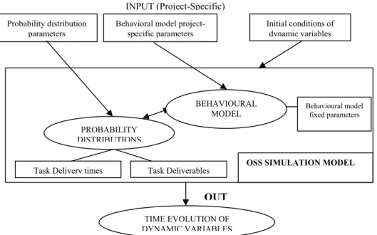
Fig. 1. General structure of an OSS dynamic simulation model.

In figure 1 we show the structure of a generic OSS dynamic simulation model. Just as in any simulation model of a dynamical system, the user must specify on input a) values to project-specific time-constant parameters, b) initial conditions for the pro-ject dynamic variables. On output, the simulation model yields the future evolution of the dynamic variables. Project-specific parameters are (i) parameters related with project outputs (eg. mean and standard deviation of LOC written by a single pro-grammer per calendar day, mean and standard deviation of defects contained per 1,000 LOC added by a programmer, mean and standard deviation of number of de-fects reported per day by a programmer, etc.) and (ii) parameters related to the

behav-Probability distribution parameters

Behavioral model project-specific parameters Initial conditions of dynamic variables INPUT (Project-Specific) TIME EVOLUTION OF DYNAMIC VARIABLES PROBABILITY DISTRIBUTIONS

Task Delivery times Task Deliverables

Behavioural model fixed parameters BEHAVIOURAL

MODEL

OSS SIMULATION MODEL

ioral model (eg. dependence of programmer interest on rate of growth of project, dependence of programmer interest on frequency of production releases, dependence of programmer interest to contribute again based on how often he/she contributed in the past etc.) These values are not precisely known from project start. One may at-tempt to provide rough estimates for these values based on results of other (similar) real-world OSS projects. However, these values may be readjusted in the course of evolution of the simulated project as real data becomes available. The way to read-just these values would be to try to fit actual data from an initial historical period of the project to the results of the simulation for the same period. By applying this con-tinuous re-adjustment of parameters (backward propagation), the simulation should get more accurate in predicting the future evolution of the project. If this is not the case, it means that a) either some of the behavioral model qualitative rules are based on wrong assumptions for the specific type of project studied or, b) the values of behavioral model intrinsic parameters (project-independent) must be re-adjusted.

3.2 Calibration of the Model

The adjustment of behavioral model intrinsic (project-independent) parameters is the calibration procedure of the model. According to this procedure, one may introduce arbitrary values to these parameters as reasonable ‘initial guesses’. Then one would run the simulation model, re-adjusting parameter values until simulation results satis-factorily fit the results of a real-world OSS project (calibration project) in each time-window of project evolution. More than one similar type OSS projects may be used in the calibration process.

4

A Specific Candidate for a OSS Generic Simulation Model

4.1 Definitions

Project modules

A project module consists of a collection of code files that have the same general specifications.

Project tasks

Project tasks are the different type of actions that can be performed by the human parties for the development and release of the project or project parts. The tasks con-sidered are:

1. Design and submit the first release version of a new module. We call this task new module submission, and index all quantities related to it by index S. This task may refer to a submission of an alternative or more advanced version of an existing (old) module. This occurs frequently during the evolution of the most popular OSS projects.

2. Correct defects that were previously reported for a specific file. We will call this task debugging, and index all quantities related to it by index B.

3. Test a specific source file and report defects. We will call this task testing, and index all quantities related to it by index T.

4. Add functionality and/or improve an existing source file. We will call this task functional improving, and index all quantities related to it by index F.

We do not consider any coordinator specific tasks for this first version of the model (such as code screening). We assume that project coordinators can undertake any of the four tasks mentioned above.

4.2 Model equations

The dynamics of the model proceed as follows: At each project day t, there are a number of certain tasks (of type S, B, T or F) initiated per project module. It is natu-rally assumed that one single individual handles each initiated task.

For each initiated task the model calculates: 1) the exact time period (in days) that it will take for the results of the task to be submitted to the development release 2) the deliverables of each task.

In order to quantify the above dynamical procedure three major sets of model equations are employed:

1. Equation set 1: It yields the number of tasks initiated at project day t per task type, per project module.

2. Equation set 2: It yields the specific results of each task (number of LOC, number of defects, defect corrections etc.)

3. Equation set 3: It yields the time period needed for each task to be completed. Equation Set 1:

Equation set 1 realizes the model mechanism for a) calculating the number of avail-able individuals E(t) that will show an initial (tentative) interest to contribute to the project in any task starting at day t, b) determining the precise way by which all or a subset of these initially interested individuals will be distributed among the (i) differ-ent task types and (ii) differdiffer-ent project modules (and/or alternative modules).

Equation 1.1: Determination of E(t).

We assume that the number of individuals that tentatively decide to contribute to the project starting at day t depends on (i) the “overall quality” of the project and (ii) the profile of the programmers that either have worked on the same project before day t or are new to the project. The “overall quality” of the project is determined by all those project-specific factors that stimulate the interest of prospective programmers leading them to decide to devote personal effort and time on any one contribution. Previous studies have pinpointed such factors as:

1. The rate of evolution of the project (the faster a project grows the more people are interested to contribute) (Crowston & Scozzi 2002).

2. The specific nature of the project (popular OSS projects tend to be those which promise to have the widest possible user base) [12],

3. The specific managerial model used by the project’s coordinating group (e.g. the frequency of production releases and the screening process for accepting a contri-bution). Usually, the more frequent a project releases [1, 9] and the less stringent the screening process [9], the higher the interest for participation in the project. 4. The participation of ‘celebrities’ widely known within the programmer (hacker)

community. If a renowned programmer is publicly known to participate in an OSS project the interest in this project receives a significant upward boost in the size of its programmer base. [12].

Taking into account all of the above factors (a)-(d) we define a time-dependent overall quality factor Q(t), which increases logarithmically with

the percentage increase per unit time in the LOC (Lines of Code), R(t), from the last production release to the one before the last,

the cumulative time average rate of change in total LOC, <∆L(t)>, in the current development release from one day to the next,

the cumulative time average of the Activity in the project, <A(t)>, which is defined as the total number of tasks that were terminated on day t.

the ‘interest boost factor’ J(t), which is zero for all t, except for the day(s) when there is an extra boost in the interest (e.g. due to the public announcement that a renowned programmer participates in the project).

Except for the overall project ‘quality’ Q(t), the number of individuals that show an interest to initiate a task depends also on the programmer’s profile. Project contribu-tors are divided into two categories: “core” contribucontribu-tors and “normal” contribucontribu-tors. It is assumed that up to a certain number of man-days so, spent on the project by any contributor, interest to contribute again increases, whereas beyond this number (s>so) interest decreases. Finally, ‘core’ contributors always show the same interest to con-tribute again independent on project quality or the amount of time they concon-tributed in the past.

Based on the above discussion, E(t) is given by the following equation:

)

(

'

)

(

)

(

)

(

t

Q

t

t

N

t

E

=

Λ

+

_core (1)

where N’core(t) is the number of available core programmers at day t and Λ(t) is a factor determining the variation of programmer interest according to programmer profile, as described above. The core programmers are assumed always to show the same interest in the project independent of its quality and their past contributions (last term in (1)).

In order to determine E at t=to, where to is the first day of he project after which simulation will apply, we set, by definition, Q=1 at t=to, assuming that we use the first to days of the real-world project to set the average values of the quantities presented in the bullets above. Then, we let E(to)=No, where we define No as the average num-ber of tasks actually performed per day as measured in the first to days of the project. For the Apache project, for example, this number was 9.8 contributions per day (av-erage over a three year period. Unfortunately, the case study did not report how this number varied with time). This completes the calibration procedure of equation 1.

Equation 1.2: Determination of number of tasks initiated for each task type and each project module.

The E(t) individuals, who have decided to contribute to the project starting at day t, will then have a closer look at what in particular they can do. It is not necessary for all of them to actually initiate a task, as they may lose interest after they browse the project site in search for an interesting assignment.

Denoting by upper index j=S,B,T,F, the task type, first lower index i=1,2,…,M, the particular project module and second lower index k=1,2,…,Si, possible alternatives of module i that an individual may contribute to, we define

P

_ikj(t) as the number of tasks actually initiated for project module i, alternative k (of module i) and task type j at day t.

In order to determine the

P

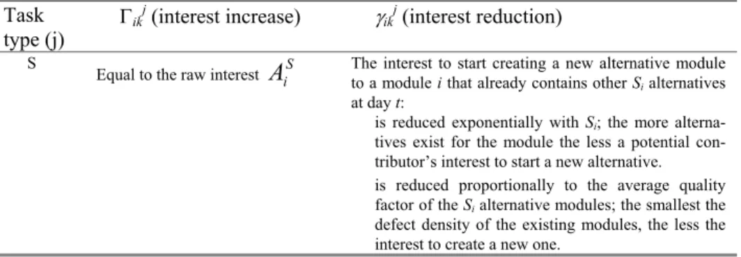
_ikj’s at every project day t, we first define the program-mer raw interest Aij for each task type j and specific module i as the ratio of contribu-tors that will, by priority, choose this task and module to contribute at any specific moment in the course of the OSS project development, before examining the precise status of development pertaining to the specific task and module. Then, we define the raw interest reduction coefficients aij as the maximum fraction of respective raw interest Aij that may be lost after prospective contributors examine the precise status of development pertaining to the task type j and module i. The Aij’s isolate a pro-grammer’s interest in a specific task based only on his/her personal preferences and independently of any specific OSS project.

Next, we define two more quantities: the interest increase factors Γikj(t) and the in-terest reduction factors γikj(t) for task type j, module i and alternative k at time t. Each Γikj(t) is directly proportional to Aij. Each γikj(t) is directly proportional to Aij and aij. In addition, they all depend on the values of time dependent project variables at time t. Table 1 presents the dependence of the interest increase and interest decrease factors (Γ’s and γ’s) on various time-dependent project variables, i.e. the particular behav-ioural model assumed.

Task type (j)

Γikj (interest increase) γikj (interest reduction) S

Equal to the raw interest

A

_iS The interest to start creating a new alternative module _{to a module i that already contains other S} i alternatives at day t:

is reduced exponentially with Si; the more alterna-tives exist for the module the less a potential con-tributor’s interest to start a new alternative. is reduced proportionally to the average quality factor of the Si alternative modules; the smallest the defect density of the existing modules, the less the interest to create a new one.

B It is proportional to the ratio of reported defects for alternative k

to the total reported defects for module i, i.e.

A

_iB, is distributed among different alternatives of module i in proportion to the fraction of defects in each alterna-tive.

The interest to initiate a defect correcting task at day t, on an alternative k of module i

decreases less, the higher the quality factor of alternative k. This behavioral rule captures the fact that potential contributors will be more interested to debug an already ‘good quality’ alternative than a ‘bad quality one’.

decreases less, the fewer the number of defects that are contained in alternative k. This behavioral rule captures the fact that many potential contributors will turn away at debugging a source file that con-tains too many bugs.

T It is inversely proportional to the number of times alternative k has been tested since its last update, i.e.

A

_iT, is distributed among alternatives of a given module according to the reciprocal of the number of times each alternative has been tested since its last update.

The interest to initiate a file testing task at day t, on an alternative k of module i

decreases more, the more times a given alternative of module i has been already tested since its last up-date. The behavioral rule assumed here is that the more times an alternative has been tested, the less interested a potential contributor would be to test it again.

decreases less, the larger the total number of tests performed in the past for the entire module. This captures the behavioral rule that, if a potential con-tributor sees that many tests are being performed for a given module (i.e. the module has attracted the in-terest of others), the more inin-terested he would be to test it himself/herself.

F It is distributed equally among all

Si alternatives in module i.

The interest for initiating a functional improvement task at day t, on an alternative k of module i, increases exponentially with the absolute value of the difference of the LOC already written (Lik) from the maximum

number of LOC Limax that is expected to be written for

any alternative of module i. If Lik≥ Limax , then the

interest decrease is maximum. The behavioral rule assumed here is that the more functionally ‘complete’ a given module alternative is, the less interested a poten-tial contributor would be to add more functionality to it and vice versa.

Table 1. Description of the dependence of the interest increase and interest reduction coeffi-cients on time-dependent project variables.

We then define the total interest factor Iikj for task type j, module i and alternative k as j ik j ik j ik

I

≡

Γ

−

γ

(2)

Finally, we propose the following master equation to determine the Pikj’s at every project day t:

∑

≠

+

=

) , , ( ) , , (

)

(

)

(

)

(

)

(

)

(

k i j r q p p qr j ik j ik j ik

_I

_t

_I

_t

_t

t

E

t

P

_γ

(3)

The basic assumption behind (3) is that a proportion of the users that turn down tasks other than j, i, k will finally turn to task j, i, k with a probability proportional to the total interest in j, i, k. The values of the Γ’s and γ’s are properly normalized so that the sum of all tasks that will actually be initiated at day t for all task types, mod-ules and alternative modmod-ules in the project is at most equal to E(t).

Equation Set 2:

Equation Set 2 determines the deliverable quantities of each of the initiated tasks by drawing from probability distributions. We use lognormal distributions, since rele-vant quantities are all positive. The following time-constant project- specific quanti-ties must be provided as initial input to the simulation model:

S i L S i

L

,

σ

: The mean and standard deviation for the number of LOC added per con-tribution for a given module i

F i L F i

L

,

σ

: The mean and standard deviation for the number of LOC added per contribution for a functional improvement (update) of an existing source file in mod-ule i.

i d i

d

,

σ

: The mean and standard deviation of the initial defect density (number of defects per LOC) of code written and submitted by a contributor for module i in a single check-in.

i T i

T

,

σ

: The mean and standard deviation of the fraction of defects in a source file of module i that are reported by a contributor undertaking a testing task.

One can obtain reasonable initial estimates for the above parameters by using real results from a known OSS and periodically re-adjusting their values at later project times by the backward-propagation procedure described in section 5.1.

Equation Set 3:

Finally, the delivery time of each initiated task is also drawn from lognormal prob-ability distributions. The following time-constant project-specific quantities must be provided as initial input to the simulation model:

S i t S i

t

,

σ

: The mean and standard deviation for the time (in days) to write one LOC for a file in module i.

B i t B i

t

,

σ

: The mean and standard deviation for the time (in days) to correct a sin-gle defect in 1,000 LOC.

T i t T i

t

,

σ

: The mean and standard deviation of the time (in days) to test the most recent version of the project’s development release and report detected defects for a file in module i, when the file contains 1,000 LOC and the development release Mx1,000 LOC (M is the number of modules of the project).

Equations Sets (1)-(3) fully determine the dynamics of the system. Due to the sto-chastic character of equation sets 2 and 3, each run has to be repeated an adequate

number of times with different random number generator seeds. Averages and stan-dard deviations of output variables must be calculated at each time step.

5

Computational Experiments and Results

We used the Apache case study as a test bed for an initial demonstration of the model’s ability to simulate the evolution of real-world projects. Unfortunately, the Apache case study, as well as other case studies available in literature, lack critical data that are needed for such a model to be accurately calibrated and validated. For certain project parameters, for which we had no data from either projects, we had to make our own plausible assumptions. Case studies conducted with the purpose of feeding the necessary data into a dynamical simulation more completely are needed so that such a model can be fully validated.

Simulation input

The exact input values of model parameters that were deduced from the Apache case study are not presented here for brevity. They were presented in detail in [11]. Results after 1,094 project days and comparison to Apache case study

Keeping all the above values fixed, we performed some initial runs by giving some initial values to the raw interest coefficients and raw interest reduction coefficients and certain model specific constant parameters. By interactive procedure we adapted the latter values, so that the model results matched reported results for the Apache project, both for the dynamic evolution of certain variables as well as their time-averages. 100 runs with different random number generator seeds were performed and averages taken for each dynamical variable. The concluded values for the raw interest coefficients were:AiS=0.065, AiB=0.0389, AiT=0.537, AiF=0.3591, aiS=aiB=aiT=aiT=1.

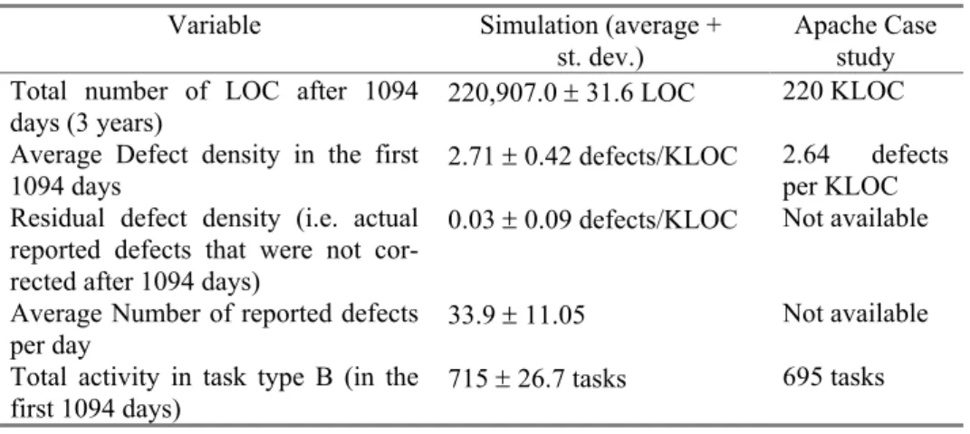
Table 2 compares average values of certain key project variables between simula-tion and reported results in the Apache project. Standard deviasimula-tions of the reported quantities as calculated after 100 simulation runs are also reported.

Variable Simulation (average +

st. dev.)

Apache Case study Total number of LOC after 1094

days (3 years) 220,907.0 ± 31.6 LOC 220 KLOC

Average Defect density in the first

1094 days 2.71 ± 0.42 defects/KLOC 2.64 defects per KLOC

Residual defect density (i.e. actual reported defects that were not cor-rected after 1094 days)

0.03 ± 0.09 defects/KLOC Not available Average Number of reported defects

per day 33.9 ± 11.05

Not available Total activity in task type B (in the

Total Activity in task type T 4,040 ± 60.9 tasks 3,975 tasks Total Activity in task type F + type S 5,991 ± 83.2 6,092 Total Activity in all task types 10,747 ± 106.5 10,762 Number of individual contributors 489 ± 21.8 388

Table 2. Comparison between simulation average results and data given in the Apache case study. Simulation results correspond to averages and standard deviations after 100 runs

Temporal evolution of project variables

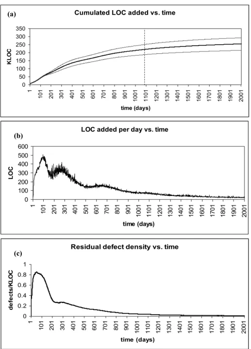
In Figures 2-3 the dynamical evolution of project variables is shown for 2,000 days. The Apache case study results pertain to the first 3 years (1,094 days) of the project, but we continued the runs in order to look at the simulated evolution at later times. For all figures, except for 2b, average data for the 100 runs is further ‘smoothed’ by taking running (window) time averages within a running window of 30 days.

Figure 2a shows the evolution of the total number of LOC added (for all project modules). The bold line shows the average of the 100 runs tried and the two dashed lines show the bounds of 1 standard deviation above and below average. We see that in the first 310 days the project reaches already half the size (110 KLOC) of the num-ber of LOC after 1094 days. Only about 35 KLOC are added from day 1095 until day 2,000. This means that project size growth rate rises at the first stages and slows down towards later stages of the OSS project. This fact is more clearly demonstrated by Figure 2b which shows the average rate of adding LOC each project day. The rate reaches a maximum around day 100 and subsequently drops. This behavior has been observed with certain strands (core) of the GNOME project and certain modules of the LINUX project.

The (almost) periodical peaks appearing in the total LOC growth rate is an interest-ing feature of the model. They are centered around the most probable dates when either a new alternative module appears in the development release, which gives a boost to functional improving tasks, or a new production release is out, which gives a boost to programmers’ interest. Finally, Figure 2c shows the evolution of residual defect density, i.e. defects per KLOC that are left unfixed. We see that the density rises rapidly in the beginning, when a lot of code is added, and defect correction ac-tivity cannot keep up. Fortunately, the model predicts that defect density will drop to the point that less than 0.1 defects per KLOC are left after day 1,000. This agrees with the Apache, FreeBSD and Linux case studies which state that defect correction is quite effective in OSS projects.

Finally, Figure 3 pertains to individual programmers. Figure 3a shows the number of “new” programmers each day that begin a task for the first time. Figure 3b is the cumulated number of new programmers. At day 1094, there is a total of 489 ± 21.8 individual programmers that have performed at least one task for the project. Com-pared to the actual number for Apache which is 388, this is indeed larger, but the disagreement is surprisingly satisfactory, if one considers that Q was calibrated using only the reported 3-year period time average values for the evolution of project vari-ables in the Apache case study and that many other data used for adjustment of model parameters was either assumed or picked from other cases studies.

Cumulated LOC added vs. time 0 50 100 150 200 250 300 350 1 101 201 301 401 501 601 701 801 901 _{1001 1101 1201 1301 1401 1501 1601 1701 1801 1901 2001} time (days) KL O C

LOC added per day vs. time

0 100 200 300 400 500 600 1 101 201 301 401 501 601 701 801 901 _{1001 1101 1201 1301 1401 1501 1601 1701 1801 1901 2001} time (days) LO C

Residual defect density vs. time

0 0.2 0.4 0.6 0.8 1 1 10 1 20 1 30 1 40 1 50 1 60 1 70 1 80 1 90 1 10 01 11 01 12 01 13 01 14 01 15 01 16 01 17 01 18 01 19 01 20 01 time (days) de fe c ts /K L O C

Fig. 2. (a) Total number of LOC cumulated vs time. The bold line is the average of the 100 runs. The gray lines are one standard deviation above and below the average. The dashed

verti-cal line shows the day of the project until data was reported in the Apache case study [8]. (b) Total number of LOC added per day. (c) Density of unfixed defects as a function of time.

(b)

(c) (a)

New programmers per day vs. time 0 2 4 6 8 10 12 14 1 10 1 20 1 30 1 40 1 50 1 60 1 70 1 80 1 90 1 10 01 11 01 12 01 13 01 14 01 15 01 16 01 17 01 18 01 19 01 20 01 time (days) Nu m . o f in d iv u d u a ls

Cumulated new programmers vs. time

0 100 200 300 400 500 600 700 800 1 10 1 20 1 30 1 40 1 50 1 60 1 70 1 80 1 90 1 100 1 110 1 120 1 130 1 140 1 150 1 160 1 170 1 180 1 190 1 200 1 time (days) N u m . of i n di v u du a ls

Fig. 3. (a) Number of new contributors per day. (b) Cumulated number of contributors vs. time.

6

Conclusions

We presented a general framework for the production of OSS dynamic simulation models. We then presented a specific simulation model for the OSS development process and attempted to produce some indicative simulation results, applying the model to the Apache case study.

Qualitatively, the simulation results demonstrated the super-linear project growth at the initial stages, the saturation of project growth at later stages and the effective defect correction, facts that agree with known studies.

Due to the lack of adequate literature data, simulation results presented here cannot be considered at all as full-scale validation of the model, a task that would require future OSS case studies conducted in parallel with the application of the simulation model, in order for all the necessary data to be available.

(a)

The simulation results, on the other hand, demonstrated the model’s ability to cap-ture reported qualitative feacap-tures of OSS. Fucap-ture work should center on

Designing alternative OSS simulation models within the general framework de-scribed in section 3,

Conducting future case studies on OSS real-world projects with the purpose of collecting all the necessary data needed for accurately calibrating and validating OSS simulation models.

References

1. Raymond E.S.: The Cathedral and the Bazaar, (1998), http://www.tuxedo.org/esr/writings/ cathedral-bazaar

2. Feller J., Fitzgerald B.: A Framework Analysis of the Open Source Software Development Paradigm. ICIS (1999) 58, http://citeseer.nj.nec.com/feller00framework.html

3. Bollinger T., Nelson R., Self K.M., Turnbull S.J.: Open-Source Methods: Peering Through the Clutter, IEEE Software 16(4):8-11 (1999)

4. McConnell S.: Open Source Methodology: Ready for Prime Time? IEEE Software 16(4):6-8 (1999)

5. O’Reilly T.: Lessons from Open-Source Software Development. Communications of the ACM 42(4):33-37 (1999)

6. Wilson G.: Is the Open-Source Community Setting a Bad Example? IEEE Software 16(1): 23-25 (1999)

7. Godfrey M.W., Qiang Tu: Evolution in Open Source Software: a Case Study. (Proceedings International Conference on Software Maintenance (ICSM) (2000)

8. Mockus A., Fielding R., Herbsleb J.: A Case Study of Open Source Software Develop-ment: the Apache Server. Proceedings International Conference on Software Engineering

(2000)

9. Jorgensen N.: Incremental Software Development in the FreeBSD Open Source Project.

Information Systems Journal 11:321 (2001)

10. Koch S., Schneider G.: Results from Software Engineering Research into Open Source Development Projects Using Public Data, Diskussionspapiere zum Taetigkeitsfeld Informa-tionsverarbeitung und InformationswirtschaftNr. 22, wiertschaftsuniversitaet Wien (2000). 11. Antoniades I.P., Stamelos I., Angelis L., Bleris G.L.: A Novel Simulation Model for the

Development Process of Open Source Software Projects. International Journal of Software Process: Improvement and Practise (SPIP), special issue on Software Process Simulation and Modelling (2003)

12. Crowston K., Scozzi B.: Open Source Software Projects as Virtual Organizations: Compe-tency Rallying for Software Development, IEE Proceedings – Software Engineering 149 (1):3 (2002)