STRUCTURE AND DYNAMICS STUDIES USING NUCLEAR MAGNETIC RESONANCE: FROM SIMPLE LIQUIDS TO EXTREME NETWORKS
Leah Marie Heist
A dissertation submitted to the faculty at the University of North Carolina at Chapel Hill in partial fulfillment of the requirements for the degree of Doctor of Philosophy in the
Department of Chemistry.
Chapel Hill 2015
ABSTRACT
Leah Marie Heist: Structure and Dynamics Studies Using Nuclear Magnetic Resonance: From Simple Liquids to Extreme Networks
(Under the direction of Edward T. Samulski)
Nuclear magnetic resonance is a powerful analytical tool utilized by chemists and biochemists to extract structural information. However, NMR has utility beyond structure determination: it is also a powerful technique for interrogating dynamics at the microscopic level. In this thesis, I have used NMR to study a diverse range of fluid systems:
liquid state structure in molecular liquids using very high field NMR orientational order in nonlinear liquid crystal dimers
molecular dynamics and structure in highly grafted “bottle-brush polymers” high performance liquid crystal thermosetting polymers.
NMR detects small changes in the magnetic energy of nuclei in different
The incompletely averaged, anisotropic NMR interactions described in Chapter 2 for simple isotropic liquidsare significant for anisotropic molecules (liquid crystals). One type of liquid crystal, the nematic phase, is characterized by molecules that tend to align their long axis on average parallel to one another in the fluid, but have no spatial correlations—no positional order. In Chapter 3, I attempt to describe the nature of a new nematic phase found in nonlinear liquid crystal dimers, introduced in 1991 by Hiro Toriumi, professor of
chemistry at Tokyo University, by supplementing recent simulation data from Photinos and coworkers at the University of Patras with extensive 2H and 13C NMR studies.
ACKNOWLEDGMENTS
My time at UNC has truly been a rewarding experience and I want to begin by thanking just some of the numerous people who have helped me along the way. First, I owe immense gratitude to my research advisor and mentor, Prof. Edward Samulski, who provided a wonderful environment to conduct research, constantly encouraged me to pursue my own ideas, and was always eager to discuss my results. Ed’s extraordinary ability to think, write, and communicate science made him a wonderful mentor and he encouraged me to live up to this high standard. I also want to thank Ed’s wife, Carol (an extraordinary writer and
communicator herself), for her friendship and invaluable advice over the years. Additionally, my gratitude goes to my committee members Prof. Sergei Sheiko, Prof. James Jorgenson, and Prof. Mark Wightman who provided me with thoughtful suggestions and insights. I am glad to have Prof. Louis Madsen (Virginia Tech) join my committee; he generated my excitement for NMR and liquid crystals and as an undergraduate he made me feel like an invaluable member of his lab.
At Virginia Tech I also had the privilege of being a member of Prof. Webster Santos’ lab. I want to thank him for being the first person to encourage me to do research and giving me a great experience in his lab. I also want to thank my high school chemistry teacher, Mrs. Stromwall. She was a compassionate teacher and I always loved going to her class.
the intricacies of NMR and Collin McKinney (Electronics) for his many hours helping me set up a power supply for my high temperature NMR probe. I also want to thank Dr. Kevin Knagge (DHMRI) for helping to secure high field NMR data.
To the many collaborators that I have worked with during my time here: I want to thank you for your scientific curiosity and for enriching my knowledge in a wide range of topics: Prof. Demetri Photinos (University of Patras), Prof. Chi-Duen Poon (UNC), Prof. Jim Emsley (Southampton), Prof. Jukka Jokisaari (Oulu), and Prof. Moreno Lelli (ENS Lyon). Many people provided samples and were invaluable resources to me: Georg Mehl (Hull) who provided the cyanobiphenyl dimer samples and Krzysztof Matyjaszewski and Joanna
Burdyńska who synthesized the labeled bottlebrushes. Lastly, to Theo Dingemans (TU Delft), an exceptional polymer chemist, who provided all the liquid crystal and LCT samples and who agreed to be on my orals committee.
Most importantly, I want to thank all of my family and friends who have been important parts of my life. Amy, thank you for being my best friend since the 2nd grade. Sarah, I am so glad we both decided to join the chemistry fraternity so we could become great friends. To my grandparents, thank you for your love and support and for being such a large part of my life. To my parents, I owe so much of my success to you for being a great example and for always wanting the best for me. Thank you for loving me and always giving me the confidence to pursue my dreams. To my husband, Chris, I am so blessed to have you in my life and I cannot wait to see what the future brings us. Thank you for always
TABLE OF CONTENTS
LIST OF TABLES ... xi
LIST OF FIGURES ... xii
CHAPTER 1: INTRODUCTION ...1
1.1 Introduction ...1
1.2 Liquid Crystals ...1
1.3 Polymer Networks ...2
1.4 NMR Theory (Nuclear Spin Hamiltonian) ...3
1.4.1 Quadrupolar Interaction ... 4
1.4.2 Spin Relaxation ... 5
1.4.3 Chemical Shift ... 7
CHAPTER 2: LIQUID STATE STRUCTURE VIA VERY HIGH-FIELD NMR ...9
2.1 Introduction ...9
2.2 High Field 2H NMR Magnetic Field Induced Alignment of Deuterated Liquids..11
2.2.1 2H NMR of Benzene at 1 GHz ... 15
2.3 Relation of Order Parameters to Molecular Pair Correlations in a Liquid in a High Magnetic Field ...19
2.4 Evaluation of Correlation Factors from Measured Spectra ...23
2.4.1 Binary mixtures (Case 1) ... 24
2.4.1.1 Benzene in TMS ... 26
2.4.1.2 Chloroform in TMS ... 27
2.4.2.1 Benzene:hexafluorobenzene 1:1 mixture in TMS ... 30
2.4.2.2 Chloroform:benzene 1:1 mixture ... 32
2.4.3 Binary mixtures (Case 3) ... 33
2.4.3.1 Thiophene in TMS ... 33
2.5 Calculated correlation factors from molecular dynamics simulations ...35
2.5.1 Benzene-benzene pair correlations ... 35
2.5.2 Chloroform-chloroform pair correlations ... 39
2.5.3 The benzene/hexafluorobenzene complex ... 40
2.5.4 Insights from chloroform-d/benzene mixtures... 43
2.6 Conclusions ...44
CHAPTER 3: NX PHASE OF CYANOBIPHENYL DIMERS ...46
3.1 Introduction ...46
3.1.2 Chiral phases ... 48
3.1.3 Nematic phases of non-linear cyanobiphenyl dimers ... 49
3.1.4 Experimental determination of the twist-bend nematic phase ... 51
3.1.4.1 Microscopy (FFTEM, Optical Microscopy) ... 51
3.1.4.2 Elastic constants in nematic phases ... 53
3.1.4.3 Experimental determination of chirality ... 55
3.1.5 An alternative structure for the NX phase of odd cyanobiphenyl dimers ... 56
3.2 Experimental Methods ...60
3.2.1 Materials ... 60
3.2.2 NMR Methods ... 61
3.3 Results and Discussion ...62
3.3.2 Deuterated probes dissolved in liquid crystals... 62
3.3.3 Comparison with chiral nematics... 68
3.3.4 Demonstration of the odd-even effect of cyanobiphenyl dimers ... 70
3.3.5 Core order parameters ... 71
3.3.6 Direct determination of Score using the chemical shift anisotropy of 13C 72 3.3.7 13C NMR of cyanobiphenyl dimers ... 74
3.4 Conclusions ...78
CHAPTER 4: LOCAL DYNAMICS OF BOTTLEBRUSH MACROMOLECULES VIA 2H NMR ...80
4.1 Introduction ...80
4.2 Experimental Methods ...82
4.2.2 NMR Methods ... 83
4.3 Results and Discussion ...85
4.3.1 Solution Dynamics in Bottlebrush Backbone ... 85
4.3.2 Solution Dynamics in Bottlebrush Macromolecules ... 88
4.3.3 Bottlebrush Dynamics Inferred from NMR Linewidths ... 90
4.4 Conclusion ...94
CHAPTER 5: LIQUID CRYSTAL THERMOSETS: HIGH PERFORMANCE THERMOSET RESINS ...96
5.1 Introduction ...96
5.1.1 High Performance Polymers ... 96
5.1.2 Current Polymer Matrix Composites ... 98
5.1.3 High Performance Thermosets ... 98
5.1.3.1 Liquid Crystal Thermosets ... 99
5.1.4. Curing of phenylethynyl based systems ... 101
5.2.1 Solid State 13C NMR ... 104
5.3 Results and Discussion ...108
5.3.1 Solid-State Spectra of LCT oligomer precursor ... 108
5.3.2 NMR of Liquid Crystal Thermosets ... 112
5.3.2.1 Chemical Shift Anisotropy in Liquid Crystals... 116
5.3.3. Exploitation of Chemical Shift Anisotropy in LCTs ... 122
5.3.3.1 LCT Model Compounds ... 123
5.3.2 Curing Kinetics ... 124
5.4 Conclusions ...127
APPENDIX A: TABLES OF 2H AND 13C NMR DATA OF CYANOBIPHENYL DIMERS ...128
LIST OF TABLES
Table 2.1. Quadrupolar splitting and Δ(Δν) for Figures 2.1-3. ... 18 Table 2.2. Constants used in the determination of correlation factors for benzene,
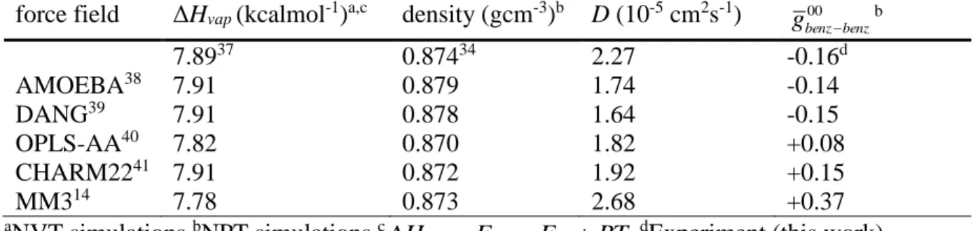
chloroform, and thiophene. ... 24 Table 2.3. Calculated radial integral of leading tensor component of g
12r
with typicalexperimental constants used to discriminate force fields (ΔHvap, density, and diffusion coefficient, D) for benzene. ... 36 Table 4. Results of toy model for benzene. ... 38 Table 2.4. Calculated radial integral of leading tensor component of g
12r
with typicalexperimental constants used to discriminate force fields (ΔHvap, density, and diffusion coefficient, D) for chloroform. ... 39 Table 3.1. Calculated values of a and b in ppm for each 13C nucleus in the phenyl rings and
CN group of 5-CB. ... 74 Table 4.1. Relaxation data for decreasing concentrations of BBBs (Br600)-d4. ... 87
LIST OF FIGURES
Figure 1.1. Three categorical shapes: calamitic, nonlinear, and discotic, representing liquid crystals with primary structures, secondary structures, and idealized shapes. ... 2 Figure 2.0. Some contents of this chapter and additional information appear in two
publications in Journal of Magnetic Resonance and Journal of Physical Chemistry Letters. ... 9 Figure 2.1. The molecular axes system for benzene, chloroform, and thiophene. ... 15 Figure 2.2. 2H spectra at 153.553 MHz of neat C6D6 ... 16
Figure 2.3. 2H – {1H} spectrum at 153.553 MHz of deuterium nuclei present at natural
abundance in neat C6H6 ... 18
Figure 2.4. Observed Δν/ν0 versus x, the mole fraction of benzene-d6 and chloroform-d in the
diluent TMS ... 26 Figure 2.5. 2H NMR spectrum of neat benzene-d6 recorded at 22.3 T (Bruker Avance III 950
MHz proton NMR spectrometer at temperature, T = 303 K). ... 27 Figure 2.6. 2H NMR spectrum of neat chloroform-d recorded at 22.3 T (Bruker Avance III
950 MHz proton NMR spectrometer at temperature, T = 303 K). ... 29 Figure 2.7. Observed Δν/ν0 versus x, the mole fraction of benzene-d6 and hexafluorobenzene
diluent TMS ... 30 Figure 2.8. 2H NMR spectrum of neat 1:1 mixture of benzene-d
6/hexafluorobenzene (no
TMS) recorded at 22.3 T (Bruker Avance III 950 MHz proton NMR spectrometer at temperature, T = 303 K). ... 31 Figure 2.9. 2H NMR spectrum of neat 1:1 mixture of chloform-d/benzene (no TMS)
recorded at 22.3 T (Bruker Avance III 950 MHz proton NMR spectrometer at
temperature, T = 303 K). ... 32 Figure 2.10. 2H NMR spectrum of thiophene-d4 (deuterons 6,9 and 7,8 labeled) recorded at
22.3 T (Bruker Avance III 950 MHz proton NMR spectrometer at temperature, T = 303 K). ... 34 Figure 2.11. Concentration dependence of thiophene pair correlation factors versus x, the
mole fraction of thiophene-d4 in TMS. ... 35
Figure 2.12. Spatial distribution function of benzene calculated with MD simulation using the AMOEBA force field. The two most probable dimer states are mutually
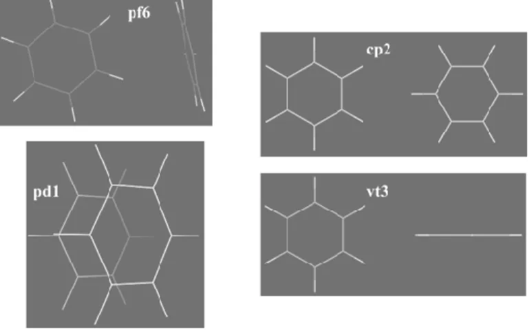
Figure 2.13. The four possible dimer configurations for two benzene molecules. ... 38 Figure 2.14. Spatial distribution function of chloroform calculated with MD simulation using
the AMOEBA force field. The two most probable dimer states are parallel
1,2 0
and antiparallel
1,2 180
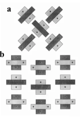
. ... 40Figure 2.15. Schematic representation of the crystal structure between (a) identical
quadrupolar molecules and (b) two quadrupolar molecules with opposite quadrupole moment configurations ... 41 Figure 2.16. Spatial distribution function of chloroform calculated with MD simulation using
the AMOEBA force field. The most probable dimer state is overwhelming parallel
1,2 0
. ... 43Figure 3.1. Examples of phases formed from calamitic mesogens: uniaxial nematic (N), uniaxial smectic-A (SA) and biaxial smectic-C (SC). ... 47
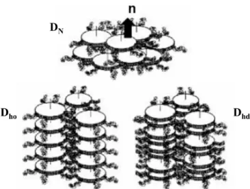
Figure 3.2. Examples of phases formed from discostic mesogens: nematic (DN), hexagonal
ordered (Dho), and hexagonal disordered (Dhd). ... 48
Figure 3.3. Approximate shape of a non-linear liquid crystal dimer and structure of CB-C7-CB. ... 49 Figure 3.4a. Uniaxial nematic phase, N, b. twist-bend nematic phase, NTB, and c. chiral
nematic phase, N* ... 51 Figure 3.5a. Schierlen texture of the uniaxial nematic phase of a liquid crystal (N) b. Focal
conic texture of the chiral nematic phase of a liquid crystal (N*) when viewed under a polarizing optical microscope ... 53 Figure 3.6. Structure and phase transition map for M2. ... 54 Figure 3.7. Prochiral molecule where X and Y substituents are different. ... 55 Figure 3.8. AFM images of (left) the NX phase showing a focal conic domain covered with
layers spaced ~8nm apart with the crystallographic structure (right) the crystalline phase showing clear evidence of 8.3 nm periodicity of the crystallographic planes. . 57 Figure 3.9a. 2H NMR of the N
X phase of deuterated CB-C9-CB (pictured) before (red) and
immediately after (blue) rotation of the sample by 90°. b. A hypothetical picture of the proposed twist-bend confirmation undergoing a rotation by 90°. ... 59 Figure 3.10. Chemical structure and respective transition temperatures of CB-Cn-CB for
Figure 3.12. Inverse gated 1H decoupled 13C NMR pulse sequence. ... 62 Figure 3.13. 2H NMR spectra of decane-d22 in CB-C11-CB at decreasing temperatures ... 63
Figure 3.14. The temperature dependence (in reduced temperature) of the quadrupole
splitting of the methyl and methylene group of decane-d22 in CB-C11-CB ... 64
Figure 3.15. 2H NMR spectra of decane-d22 in CB-C9-CB at decreasing temperatures ... 65
Figure 3.16. The temperature dependence (in reduced temperature) of the quadrupole
splitting of the methyl and methylene group of decane-d22 in CB-C9-CB ... 65
Figure 3.17. 2H NMR spectra of decane-d22 in CB-C7-CB at decreasing temperatures ... 66
Figure 3.18. The temperature dependence (in reduced temperature) of the quadrupole
splitting of the methyl and methylene group of decane-d22 in CB-C7-CB ... 67
Figure 3.19. A possible arrangement of mesogenic units within each chiral domain for odd cyanobiphenyl dimers. ... 68 Figure 3.20. 2H spectra of 2 wt% decane-d
22 dissolved in cholesteryl nonanoate (CN) cooled
into the smectic phase and heated to access the cholesteric phase ... 69 Figure 3.21. The temperature dependence (in reduced temperature) of the quadrupole
splitting of the α-methylene group of decane-d22 in all samples including the
monomer, 5-CB and the even dimer, CB-C10-CB. ... 71 Figure 3.22. 13C spectra of CB-C11-CB at decreasing temperature with 1H decoupling. ... 75 Figure 3.23. 13C spectra of CB-C11-CB at decreasing temperature without 1H decoupling. 76 Figure 3.24. The temperature dependence (in reduced temperature) of the order parameter of CNin CB-C11-CB, CB-C9-CB, CB-C7-CB, and the monomer 5-CB... 77 Figure 3.25. 13C NMR of CB-C10-CB in the nematic phase. ... 78 Figure 4.1. Schematic diagram of bottlebrush macromolecule (BBM) showing label in
backbone, grafted “bristles” and “hair” on each of the bristles. ... 81 Figure 4.2 The synthetic pathway for the preparation of a. ATRP diinitiator-d4 (Br-d4-Br)
and b. labeled BBMs and PnBA side chains ((600-g-5/44)-d4). ... 83
Figure 4.3. Inversion recovery pulse sequence. Values of τ are varied for measuring the spin-lattice relaxation time, T1. ... 84
Figure 4.4. Car-Purcel-Meiboom-Gill (CPMG) pulse sequence. Values of n are varied for measuring the spin-spin relaxation time, T2. ... 84
Figure 4.6. 2H 1D NMR spectra of (Br600)-d4 (0.09g/mL in DCM), (600-g-5)-d4 (10 wt% in
DCM), and (600-g-44)-d4 (12 wt% in DCM). ... 87
Figure 4.7. Experimental data for determination of T1 (a) and T2 (b) for three concentrations
of BBB. Shaded line represents the estimated error in the exponential fit. ... 88 Figure 4.8. Experimental and simulated spectra of the bottle-brush (600-g-44)-d4 in DCM. 92
Figure 4.9. Experimental and simulated spectra of the neat bottle-brush (600-g-5)-d4 ... 94
Figure 5.1a. All-aromatic high performance polymers and b. melt processable high
performance polymers. ... 97 Figure 5.2 The LCP VectraTM. ... 99 Figure 5.3 LCT reactive oligmer... 100 Figure 5.4. Liquid crystal thermoset a. before and b. after curing with preferred direction
along n. ... 100 Figure 5.5. 1H broadband decoupling 13C NMR pulse sequence using cross polarization .. 102
Figure 5.6. 1H broadband decoupled 13C pulse sequence. ... 103 Figure 5.7. Home-built oven for 13C NMR probe capable of reaching over 400°C. ... 104 Figure 5.8. 13C powder pattern of the LCT precursor oligomer ... 105 Figure 5.9. Representative, idealized spectra from single crystals with one orientation (left)
and powders with random orientations (right). From ref 3. ... 106 Figure 5.10. 13C NMR spectra of the LCT oligomer. ... 108 Figure 5.11. 1H broadband decoupled 13C CP/MAS spectrum of a. HBA, b. HNA, c.
PE-COOH, and d. PE-OAc ... 110 Figure 5.12. Sum of 13C CP/MAS spectra of HBA, HNA, PE-COOH, and PE-OAc (scaled to
ratios of monomers and end-groups). ... 111 Figure 5.13. Overlay of Figures 5.12 (sum, blue) and 5.10 (red). ... 112 Figure 5.14. Simplified picture of a liquid crystal polymer melt before and after a magnetic
field is applied. ... 113 Figure 5.15. Proposed di- (f = 2) and tri- (f = 3) functionalized cure products of the
phenylethynyl end-group chemistry. ... 114 Figure 5.16. 13C NMR spectra of 1000 g/mol LCT precursor. Isotropic CP/MAS (red)
Figure 5.17. 1H decoupled 13C spectra of TBBA in the isotropic phase and various oriented phases. ... 117 Figure 5.18. 1H decoupled 13C spectra of TBBA in the nematic phase using different 1H
decoupling schemes. ... 119 Figure 5.19. Proton-decoupling 13C NMR of 5-CB in the isotropic and nematic phases. ... 120 Figure 5.20. Dimethylacetylene structure and axes system with the z-axis along the acetylene
bond... 121 Figure 5.21. 13C spectra of DPDA-OC5 in the nematic and isotropic phases. ... 122
Figure 5.22. 13C NMR of LCT after curing at 300°C for 75 min for various time intervals 123 . A qualitative loss of the ethynyl carbon peak intensity is observed. ... 123 Figure 5.23. CP/MAS (isotropic) spectrum in red and oriented (anisotropic) spectrum in blue
of the PE-napthalenediol-PE model compound. ... 124 Figure 5.24. 13C NMR of LCT precursor model compound (PE-napthalenediol-PE).
Different durations of curing in minutes at 300°C and plot of concentration of ethynyl peak vs. cure time used to determine kinetic rate constants. ... 125 Figure 5.25. Kinetic plot of the natural log of concentration vs. cure time in minutes.
CHAPTER 1: INTRODUCTION 1.1 Introduction
Nuclear magnetic resonance (NMR) is a powerful analytical tool for studying a wide range of materials from simple liquids to complicated polymer structures and architectures both in solutions and in the solid state. Additionally, NMR provides information about structure as well as dynamics over various length and time scales.1 In this thesis, the
attributes of NMR are clearly demonstrated by studies of four very different materials: simple liquids like benzene and chloroform, nematic liquid crystals, and extreme polymer networks: very tough liquid crystal thermosets and very soft bottlebrush elastomers. A brief description of the materials considered in this thesis and the underlying NMR theory used is described.
1.2 Liquid Crystals
Figure 1.1. Three categorical shapes: calamitic, nonlinear, and discotic, representing liquid crystals with primary structures, secondary structures, and idealized shapes. From ref 2.
The most is known about phases formed from the two extreme shapes: calamitic and discotic. The primary structure is characterized by a mesogenic core, typically made up of aromatic groups, that facilitates into a fluid phase by lowering the melting temperature, Tm. The symmetry axis of the meson is represented by l. The symmetry axis of the fluid is termed the director, n. These primary molecular shapes can organize into a variety of fluid phases and some are discussed in Chapter 3 and a new nematic phase is explored.
1.3 Polymer Networks
flexible polymer chains form entanglements with their neighbors. The formation of either physical or chemical cross-links between polymer chains is generally known as gelation and results in a three-dimensional interconnected “single” macromolecule or network. The strength of these interactions determines the mechanical properties of the network. A typical property used to measure the “stiffness” is the shear modulus which describes the material’s response to shearing strains and is in units of pressure (force per sheared area). Liquids have a zero shear modulus and metals can have moduli up to hundreds of GPa. The modulus of polymeric materials falls in the middle of these two extremes; polymer networks are tailored to have moduli specific for a desired application. In Chapter 4, bottlebrush architectures forming super-soft (low modulus) elastomers are described and in Chapter 5, super-tough (high modulus) liquid crystal thermosets are described.
1.4 NMR Theory (Nuclear Spin Hamiltonian)
Nuclear spin interactions give rise to a breadth of information about chemical structure, chemical processes, and dynamics of molecules. These interactions are probed using NMR and will be used in the study of the two aforementioned polymer systems.
The quantum mechanical description of NMR uses the spin Hamiltonian to describe the various interactions involved when a sample is subjected to an external magnetic field. When this external field, B0, is applied, the energy of the nuclear magnetic moments is
perturbed. The spin Hamiltonian describes these changes in energy. The external spin Hamilton is purely magnetic and describes interactions between the spin system and the external magnetic field. This field causes the nuclear Zeeman splitting which splits spin quantum states that are normally degenerate.
J jk DD jk Q j CS j
j H H H H
The internal spin Hamiltonian (Equation 1.1 for spin j interacting with spin k) is much more complicated because it involves all other spin interactions with its environment and other spins. These include the chemical shift (CS), which attenuates the external magnetic field through the motion of the electrons in the field. The quadrupolar coupling (Q) is a result of the interaction of a quadrupolar nucleus and the local electric field gradient formed by electrons in the chemical bond to quadrupolar nuclei. Direct dipole-dipole couplings (DD) are caused by the direct magnetic interaction of nuclear spins through space. Finally, the J-coupling (J), or indirect dipole-dipole coupling, involves the spin interactions through the bonding electrons.3
1.4.1 Quadrupolar Interaction
The nuclear quadrupole coupling manifests itself in 2H NMR; deuterium has a spin quantum number of 1. The nuclear quadrupole moment of the 2H nucleus (D) strongly
interacts with the electric field gradient generated by the surrounding electron clouds (primarily the C—D bonding electrons), making it a purely intramolecular interaction. The relevant parameter is the quadrupole moment of the nucleus, which for 2H is 0.2860 x 10⁻²⁸ m2 and small enough to be observed by NMR (as opposed to nuclear quadrupole
spectroscopy).
2 3 ) 2 ˆ 3 ( 6 1 ˆ 2 zz Q z Q Q j V eQ I H (1.2)
The ωQterm is averaged over all molecular motion, so it averages to zero in isotropic liquids. Therefore, the Hamilton is zero and it does not influence the position of the NMR peaks in isotropic liquids. The quadrupolar interaction does, however, strongly influence the relaxation of nuclear spins. The relaxation for 2H nuclei is solely influenced by the
quadrupole interaction, which is purely intramolecular. Because the natural abundance of 2H
is so low (~0.015%), molecules are usually labeled with 2H at particular hydrogen positions to probe molecular dynamics by the reorientations at those labeled positions.3
1.4.2 Spin Relaxation
By 2H-labeling, the dynamics of local motion can be probed at the site of the C—D bond. This technique is used to study dynamics in polymer bottlebrushes (Chapter 4). And, by considering some simple theoretical relations, relaxation can give information about this local motion.
Spin relaxation proceeds by two different mechanisms. When an external magnetic field is introduced (B0), the spins reach thermal equilibrium where there is a slight preference
for the lower energy spin state caused by the Zeeman splitting. This causes a slight excess of magnetization parallel to the external magnetic field, which is defined to be the z-axis. When spins are subjected to this external magnetic field, they begin to precess at the Larmor
frequency, ω0, which is linearly related to the magnetic field strength (Equation 1.3) where γ
0 0 B
(1.3)
The slight excess in magnetization in the positive z-direction is given by the Boltzmann distribution (Equation 1.4).3
kT B kT
E
upper
lower e e
N
N 0
(1.4)
The spin lattice relaxation characterizes the evolution of the spin populations to thermal equilibrium in the presence of the field. It is the buildup of longitudinal spin excess population and is described by the time constant, T1. T1 is measured by an NMR experiment
known as inversion recovery in which a radiofrequency pulse effectively torques the bulk (excess) magnetization into the -z direction. The inversion recovery experiment tracks the bulk magnetization as it relaxes back to its equilibrium position along +z.
The spin-spin relaxation process has to do with the fact that the magnetization is actually measured in the transverse direction (xy-plane instead of along z). The
magnetization cannot be measured along the z-axis because the large external magnetic field, B0, is too overwhelming to measure the small magnetization caused by the spins. The NMR
experiment proceeds as follows: a radiofrequency pulse torques the magnetization into the xy-plane for detection. After some time (described by the spin-spin relaxation time T2), this
transverse magnetization decays to zero because once the radiofrequency pulse is turned off, the transverse magnetization begins to precess about the B0 field at the Larmor frequency.
However, it is impossible for the spins to maintain exact synchrony due to small fluctuations in the local field strength. This decay of the transverse magnetization to zero is described by the time constant, T2. The spin-echo experiment, which measures the decay of the NMR
1.4.3 Chemical Shift
Magnetic fields tend to vary on a sub-molecular distance scale due to the contribution of electron-generated currents. The external magnetic field induces circulating currents in the electron density distribution within molecules which, in turn, creates an additional induced and opposing (diamagnetic) magnetic field. The local magnetic field at a certain nucleus is given in Equation 1.5.3 The induced field (shielding) is about 10-4 the size of B0.
induced j loc
j B B
B 0 (1.5)
The chemical shift (δ) is described by a tensor, specifically a 3 x 3 matrix of real numbers. Typically principal axes are assigned to each nuclei that correspond to structural features of the molecule. The principal values are defined when the axis of the induced field is along the external magnetic field (Equation 1.6). Equation 1.6 applies if the external field is along the z principal axis; analogous equations can be written for j
xx
and j yy
where the external field is along the x and y principal axes, respectively. Each nuclear site has a different chemical shift tensor with a different principal axis system. All off-diagonal terms of the chemical shift tensor are zero for the principal axis system.
0
B
Binducedj zzj (1.6)
The isotropic chemical shift is the average of the 3 principal values
j
zz j yy j xx chemical shift is no longer an average over all orientations with equal probability, but biased orientations are sampled relative to B0 because in the nematic phase the molecules are
CHAPTER 2: LIQUID STATE STRUCTURE VIA VERY HIGH-FIELD NMR
Figure 2.0. Some contents of this chapter and additional information appear in two publications in Journal of Magnetic Resonance and Journal of Physical Chemistry Letters. 2.1 Introduction
Efforts to describe the structure of the liquid phase followed far behind those applied to solids and gases.5 By the 1950s, however, the liquid state received more attention and attempts to develop a theory of liquids increased.6–9 Previous work in liquid state structure
theory for a geometric model of liquid state structure and hoped that it could be adapted for computer simulations, which was steadily growing at the time.10
Molecular dynamics (MD) simulations have provided the most progress in developing a complete molecular description of the liquid state.11,12 However, computer simulations are reliant on the accuracy of the force field used. MD simulates the movement of atoms; the force field replaces true forces and potential energies between atoms with a simplified model of pairwise “atomistic” interactions.13 Force fields describing those
interactions have differing levels of complexity and the choice of force field is a balance between maximization of accuracy of simulations with minimization of computing time. As computing power has grown, force fields have improved14–16 and are continuously optimized. Optimization includes fitting simulated data to available experimental results (i.e. heat of vaporization, density, self-diffusion, X-ray, and neutron scattering) or performing quantum calculations.17 With this limited set of experimental parameters, it is often difficult to
discriminate between force fields for a given system. Therefore, it is of use to find additional experimental parameters that simulated results can be fit to in order to improve the reliability of a chosen force field. Specifically, molecular simulations benefit from experimental parameters that probe subtle intermolecular interactions.
We show that very high-field 2H nuclear magnetic resonance (NMR) yields an additional experimental parameter that discriminates against force fields. The technique uses deuterated liquids and their mixtures to extract the leading tensor component of the pair correlation function, a parameter that can readily be calculated from MD simulations. These
molecular liquids and mixtures showing that experimental parameters found using the high-field NMR method are very sensitive to the choice of simulation force high-field. This new experimental parameter is a directional probe of molecular interactions whereas many experimental parameters are dominated by isotropic interactions (i.e. density, self-diffusion, and heat of vaporization).
Herein we describe the application of high field NMR observations for the prototypical liquids benzene and chloroform, in binary and tertiary mixtures. Results are also presented for thiophene, which provides an example of less symmetric molecule and, consequently, a richer set of measurable quantities.
2.2 High Field 2H NMR Magnetic Field Induced Alignment of Deuterated Liquids
It is well understood that anisotropic liquids (liquid crystals) can align when an external field is applied. Molecular orientation in ordinary liquids, however, is less studied. With the advent of high strength magnetic fields,18 very small molecular alignments due to the molecular magnetic anisotropy—the magnetizability—can be detected with NMR by measuring associated nonzero averages of dipolar and quadrupolar interactions.
This molecular alignment effect in isotropic liquids was first described by MacLean and co-workers in 1978.19 A strong external magnetic field will align magnetically
anisotropic molecules relative to the field direction. Brownian motion of these molecules disturbs this alignment, however, so only a very small residual alignment results.20 Dipolar interactions are, relative to quadrupolar interactions, small and make detection of the
alignment in simple liquids difficult. Quadrupolar couplings are the dominant interactions in
2H NMR. The 2H nucleus has an asymmetric nuclear charge distribution (quadrupole
and the nuclear quadrupole moment perturb the Zeeman magnetic energy levels and are readily detected.3
Magnetic field-induced molecular alignment may be described by an “order parameter” given by the average,S 3/2cos
2 1/2 , where θ is the angle between the applied magnetic field direction and the principal axis of the molecular magnetizability.19The approximate alignment imposed by a magnetic field on aromatic molecules (with anisotropic magnetic magnetizability) is around S = 10-5 to 10-6. To put that in perspective, order parameters exhibited by liquid crystals in a magnetic field are between S = 10-2 and 1. The alignment of aromatic molecules studied here are similar to that experienced by polar molecules in an electric field (10-4 to 10-6).21 Although not as strong as that of liquid crystals,
these alignments are still large enough to be detected using high-resolution, high-field NMR. The alignment described is detected because of the non-zero average nuclear
interactions present in an aligning medium—a liquid crystal of merely a very high magnetic field. The complete Hamiltonian (Equation 2.1) describes the nuclear interactions in a spin system and is the sum of the Zeeman interaction (Z), the interaction between the nuclear spin and the external magnetic field and the internal interactions from Equation 1.1. 22
J jk DD jk Q j CS j Z j
j H H H H H
Hˆ ˆ ˆ ˆ ˆ ˆ (2.1)
The quadrupolar
HˆQj and dipolar
DD jkHˆ interactions are neglected in isotropic liquids due to isotropic averaging motions; however, they become apparent in NMR spectra of aligned molecules. The resonance line is split as a result of the alignment and its
From Equation 1.2, the resulting quadrupolar term of the spin Hamiltonian (Equation 2.2) is described in terms of Vz'z', the average electric field gradient formed by the electron distribution at the nucleus. The zˆ unit vector is chosen so that it is parallel to the magnetic field axis (B0) in the laboratory axis system.19
3ˆ 2
6 2 3 ˆ 2 ' ' '
zz z
Q V I
h eQ
H (2.2)
The resonance line splitting is given by Equation 2.3.19
' ' 2 3 z z V h eQ
(2.3)
The simplified expression for Vz'z' is expressed in terms of the molecular field gradients Vαβ
and the polar angles θ and φ, where θ is the angle between the zˆ and zˆ axes (Equation 2.4).21 The principal axes (xˆ,yˆ,zˆ) are chosen so that Vzz is the largest component and Vyy is the smallest component. This makes the EFG asymmetry parameter, EFG (Vxx Vyy)/Vzz, positive.
sin cos2
2 1 2 1 cos 2
3 2 2
'
'z zz xx yy
z V V V
V (2.4)
It is common to introduce a third axis system: the molecular axes aˆ,bˆ,cˆ that all deuterated sites on the molecule have in common. The molecular axis is chosen so that one of its axes is identified with the molecular symmetry axis and the other two are taken perpendicular to the symmetry planes. The molecular and local frames do not always coincide, so sometimes it is necessary to transform axes by relating Vzz and (Vxx-Vyy) in Equation 2.4 to components in the local frame where l is the direction cosine of the molecular axis α, (Vxx– Vyy)/Vzz is the
2 2 2
) ( ) ( 2 1 2 1 ) ( 2 3
eq lz lx ly
V (2.5)
In aromatic molecules (i.e. benzene), the principal molecular axis is the axis where the magnetizability is the largest (z-axis). In molecules similar to benzene this corresponds to the C6 axis of symmetry. It follows that the resonance line splitting of benzene can be described
by Equation 2.6.21
sin cos2
2 1 cos 2 3 ) 1 ( 4
3 2 2
2
c h
qQ e
v EFG (2.6)
In Equation 2.6, c is a constant that accounts for the transformation from the molecular axis to the local axis. The quadrupolar coupling constant is e2qQ/h and the angular brackets <…> denote motional averages of the direction of the magnetic field relative to the principal EFG axes at the deuterated site. The two orientational averages in Equation 2.6 are referred to as the molecular orientation order parameters, S and R, and are given in Equation 2.7.
, sin cos2
2 1 cos 2
3 2 2
R
S (2.7)
where θ is the angle of the magnetic field direction zˆ relative to the cˆ molecular axis and φ is the angle between the aˆ axis and the projection of the magnetic field direction zˆon the
b
aˆ,ˆ plane. The average term can be calculated with Boltzmann statistics (Equations 2.8 and 2.9).21 kT B2 2 15 1 2 1 cos 2
3
(2.8) kT B2 2 15 1 2 cos
In Equation 2.8, Δχ is the anisotropy of the molecular magnetizability and in Equation 2.9, δχ describes the asymmetry of the molecular magnetizability (Equation 2.10).
aa bb
aa bbcc
1/2 , (2.10)
The deuterated liquids and their mixtures studied here include benzene, chloroform, and thiophene. The molecular axes system for each is shown in Figure 2.1.
Figure 2.1. The molecular axes system for benzene, chloroform, and thiophene.
2.2.1 2H NMR of Benzene at 1 GHz
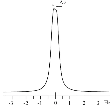
The quadrupolar splitting Δν that results from the small alignment effect in benzene-d6 is ~1 Hz at 22.3 T. We also observed the 2H NMR spectrum of benzene-d6 in a slightly
higher field spectrometer (23.4 T, 1 GHz protons) (Figure 2.2). Three split resonances are observed: the splitting of the central resonance Δν’ and two 13C satellite doublets Δν. The
magnitude of Δν’ is smaller than Δν and this difference, Δ(Δν – Δν’) is due to the unresolved fine structure; the direct dipole-dipole interactions are negligible (~0.01 Hz). In our report in Journal of Magnetic Resonance24 we determine the origins of and simulate this difference, and report pulse sequences that exploit the connectivity of the peaks in the 13C and 2H spectra to determine the relative signs of the indirect coupling, JCD, and Δν. The result: a positive
magnetic energy of the aromatic ring is lowest for configurations where the C6 axis is normal
to the field.
Figure 2.2. 2H spectra at 153.553 MHz of neat C
6D6 acquired with a standard single-pulse
sequence by using the tuned 2H lock channel and stopping the lock signal acquisition during the experiment. The low radiofrequency power allowed for the lock channel has limited the π/2 pulse to 174.0 μs (1.43 kHz), but this is sufficiently long to uniformly excite the narrow
spectral width in all of the present experiments. Both spectra were obtained averaging 64 scans with 32k complex points for an acquisition time of 8.53 s and a recycle delay of 2.0 s.
The origin of this difference, Δ(Δν), was perplexing at first because the 13C satellites
There is some variation in the splittings calculated from the direct measurement of the separation of the peak maxima, fitting the full spectrum, or fitting each doublet separately. The fitting routines were tested by generating a spectrum consisting of 6 lines centered approximately at the same positions as those in the experimental spectrum. The model spectrum had equal line separations and linewidths. The fitting routines obtained the correct line positions, and linewidths, and it was concluded that these routines were not introducing errors for the line positions. Hence, in agreement with the experimental spectra, the
magnitude of double splitting of the central line is different from those of the 13C satellite peaks.
Another proposal for the origin of this difference was that the C—D bond length differs for 13C and 12C, which impacts the quadrupolar coupling constant.25–27 However, even using dramatic estimates for bond lengths, this could not explain the difference in the quadrupolar splitting between the 13C satellites and the central peak. Another consideration was the effect of a single 13C on the molecular magnetizability tensor and its putative
influence on the molecular order tensor. The question was whether or not the presence of 13C breaks the 6-fold symmetry of benzene. However, this difference vanishes for the proton decoupled natural abundance 2H NMR spectrum of neat benzene (Figure 2.3). For this
Figure 2.3. 2H – {1H} spectrum at 153.553 MHz of deuterium nuclei present at natural abundance in neat C6H6 obtained by addition of 23168 scans as described in the text.
The spectrum was acquired using the 2H lock channel by stopping the lock acquisition during the experiment. The 2H π/2 pulse was 155.0 μs (1.61 kHz). The acquisition time was 3.2s, collecting12288 complex points. During the acquisition time a 1H WALTZ-65 decoupling at
2.77 kHz of power was applied. The recycle delay was set to 0.5 s. The magnitudes of the apparent doubles and Δ(Δν) are given in Table 2.1.
Table 2.1. Quadrupolar splitting and Δ(Δν) for Figures 2.1-3. spectrum left satellite doublet
(Hz)
center doublet (Hz)
right satellite doublet (Hz)
Δ(Δν) (Hz)
Figure 2.2 1.16 1.06 1.15 0.10±0.01
Figure 2.3 1.15 1.14 1.12 -0.02±0.02
structure for the central doublet leads to an apparent difference between the satellite splittings and that of the central doublet. This is consistent with the lower apparent resolution for the central doublet of C6D6 compared to the natural abundance 2H spectrum of C6H6.
Fortuitously, the envelope of the fine structure in the satellite doubles is an excellent
approximation to the actual quadrupolar splitting.24 For this reason, the 13C satellite doublets for benzene are used as the true quadrupolar splitting for relation to molecular pair
correlations in the remaining sections.
2.3 Relation of Order Parameters to Molecular Pair Correlations in a Liquid in a High Magnetic Field
The orienting potential of a molecule in a magnetic field with diamagnetic anisotropy tensor is on the order of 10-4kT. Starting from the formal statistical mechanics definition of the order parameter of molecule of species A in a liquid consisting of NJ molecules
...)
(NJ NANBNC SA, the first-order perturbation result is given in Equation 2.11.
...) ) 2 1 ( ) 2 1 ( )) 2 1 ( 1 ( ( 10 02 00 02 00 02 00 2
cc AC C AC
C C AB B AB cc B B AA A AA A cc A
A x g g x g g x g g
kT B
S
(2.11)
Here xJ NJ /N is the mole fraction of species J( A,B,C,...),
Jcc bb J aa Jj
/
denotes the magnetic biaxiality of the molecule and cc J bb J aa
J
, , denote the principal values
of , with Jcc 0
bb J aa
J
and the principal axes aˆ,bˆ,cˆ assigned so that
bb J aa J cc
J
. The magnetic biaxiality is zero for an axially symmetric molecule and...) ) 1 ( ( 10 00 00 00 2 AC cc C C AB cc B B AA A cc A
A x g x g x g
kT B
S (2.12)
The correlation factors expressed as 00
AJ
g are integrals of the pair correlation function )
, ;
( 1 i
AJ r
g , specifically
i i AJ i
AJ d d dr g r
V N
g
2 ; ,
1 cos 2 3 2 1 cos 2 3 8 1 2 1 2 1 2
00
(2.13)
Equivalently, these correlation factors can be directly identified with the radical integrals of the second rank function of the tensor expansion28 of the pair correlation function for axially symmetric molecules
*
2 1 2 1 2 1 2 1 21 1 1 2 2
2 1 1 2
;
; lm l m lm
l l l mmm
Y Y Y m m m l l l C r l l l g
g r
(2.14)where C
l1l2l;m1m2m
denotes the Clebsch-Gordan coefficients and Ylm is the spherical harmonics. In particular,
r g r dr
V N
gAJ00 5 2 AJ 220;00; (2.15)
Similarly, starting from the counterpart of the formal statistical mechanics definition of SA for the order parameter RA for a molecule of species A we obtain the result
... 2 1 2 1 2 1 3 2 10 22 20 22 20 22 20 2 AC C AC cc C C AB B AB cc B B AA A AA A A cc A
A x g g x g g x g g
kT B
R
, (2.16)
where the correlation factors 20
AJ
g are obtained from the Wigner expansion second rank components analogously to Equation 2.15.
The order parameter SA has a concentration independent part, which does not involve molecular pair correlations
SA B ccA /10kT2
molecule at infinite dilution. For benzene this value matches what is found in Equation 2.8. The ratio SA/
SA 0 is often29–32 expressed as a ratio
eff Acccc A
g2
/
where
ccA eff is an effective magnetizability anisotropy and g2 is the Kirkwood correlation factor, givenexplicitly in Equation 2.17 using the expression for SA found in Equation 2.11.
02 00 ,... , 0 2 2 11 cc AJ J AJ
A cc J B A J J A A g g x S S
g
(2.17)
Similarly, for magnetically biaxial molecules, the concentration independent (infinite
dilution) part of the order parameter is
RA 0
B2Acc/10kT
2/3A
(matching Equation 2.9 for benzene) and the ratio
A eff /
A where
A eff
is an effective biaxiality (Equation 2.18).
22 20 ,... , 0 2 1 2 31 AJ J AJ
B A J cc A A cc J J A eff A A
A x g g
R R (2.18)
The liquid systems studied here fall under the following symmetry categories with their respective values of SA and RA.
1. Binary mixtures where the molecules of species A are magnetically uniaxial meaning the cˆ axis is a symmetry axis with greater than twofold symmetry and molecules of species B are magnetically isotropic
Bcc 0
. This is the case for A = benzene-d6and B = tetramethylsilane (TMS) and for A = chloroform-d and B = TMS.
Expressions for the order parameters in Equations 2.11 and 2.16 reduce to Equation 2.18.1.
1
; 0 10 00 2 A AA A
cc A
A x g R
kT B
S (2.18.1)
isotropic. This is the case for A = benzene-d6, B = hexafluorobenzene (C6F6), and C =
TMS. Expressions for the order parameters in Equations 2.11 and 2.16 reduce to Equation 2.18.2. 0 ; 1 10 00 00 2
cc AB A
A cc B AA cc A
A x g g R
kT χ B S (2.18.2)
3. Binary mixtures where the molecules of species A are magnetically biaxial meaning the cˆ axis is not a symmetry axis and molecules of species B are magnetically isotropic. This is the case for A = thiophene-d4 and B = tetramethylsilane (TMS).
Expressions for the order parameters in Equations 2.11 and 2.16 reduce to Equation 2.18.3.
20 22
2 02 00 2 2 1 3 2 10 ; 2 1 1
10 A A AA A AA
cc A A AA A AA A cc A
A x g g
kT B R g g x kT B
S
(2.18.3)
In addition to the explicit dependence of SA and RA on concentration, there is an implicit concentration dependence of correlation factors. The concentration dependence on correlation factors is generally weak for the systems studied here because the measurements are taken far away from any phase transitions and can be estimated by the leading terms in the Taylor expansion. The variation with concentration x is obtained from the pure
compound (x = 1) values (Equation 2.19).
1 2 2 2 1 2 1 2 1 2 1 2 1 1 2 1 1 1 x n n AJ x n n AJ n n AJ n n AJ T g x x g x x g x g (2.19)2.4 Evaluation of Correlation Factors from Measured Spectra
In the following we present the results from the study of four mixtures: (i) benzene in TMS, (ii) chloroform in TMS, (iii) benzene/hexafluorobenzene 1:1 mixture in TMS, and (iv) thiophene in TMS. Each mixture matches one of the cases laid out in Section 2.3 (Equations 2.18.1, 2.18.2, and 2.18.3). Table 2.2 gives all of the constants used to evaluate the data and calculate the order parameters in Equations 2.18.1-3. Benzene-d6 has magnetically
Table 2.2. Constants used in the determination of correlation factors for benzene,
chloroform, and thiophene. Thiophene has inequivalent deuterons (see labeling in Figure 2.1) where deuterons 6 and 9 have their C—D bond adjacent to the sulfur atom.
molecule constant value
B 22.3 T
k 23 1
JT 10 38 .
1
T 303 K
benzene-d6 cc 7.11028JT2
aa
28 2
JT 10 6 .
3
bb
28 2
JT 10 6 .
3
EFG
0.05433
Q
1870.4kHz34
chloroform-d cc 28 2
JT 10 5 .
1
aa
28 2
JT 10 76 .
0
bb
28 2
JT 10 76 .
0
EFG
0
Q
1670.6kHz35
thiophene-d4 cc 5.71028 JT2
aa
28 2
JT 10 8 .
2
bb
28 2
JT 10 9 .
2
0.016
Q
(7,8) 190.4 kHz
EFG
(7,8) 0.058
Q
(6,9) 193.6 kHz
EFG
(6,9) 0.080
(7,8) (18034)
(6,9) 74
2.4.1 Binary mixtures (Case 1)
In the cases of benzene and chloroform mixtures with TMS (a tetrahedral,
splittings of the deuterated species at temperature T and mole fraction xA is given in Equation 2.20.
00
,
0 1
, A A AA
A T x T xg
(2.20)
where 0,A
T is the splitting of the isolated molecule (infinite dilution). According toEquations 2.3-5, the values of 0,A
T for benzene and chloroform are given in Equations 2.20.1 and 2.20.2.
EFG
cc benz Q benz kT B
T
1 10 4 3 2 , 0 (2.20.1)
kT B T cc benz Q clfm 10 2 3 2 , 0 (2.20.2)
As stated previously, there is an implicit concentration dependence of gAA00 because pair correlations depend on whether species A (here benzene or chloroform) is predominantly surrounded by molecules of species A or the magnetically isotropic diluent TMS. This concentration dependence is described in Equation 2.19 and simplified here:
00 00 2 00
00 1 2 1 1 ) 1 ( )
( AA AA AA
AA x g x x g x g
g . (2.21)
Figure 2.4. Observed Δν/ν0 versus x, the mole fraction of benzene-d6 and chloroform-d in the
diluent TMS; the respective lines are fits of Equation 2.21 to the data.
Details in this section on the benzene and chloroform analysis are given in our manuscript in the Journal of Physical Chemistry Letters.36
2.4.1.1 Benzene in TMS
According to Equation 20.1 and using the constants for benzene listed in Table 2.2,
0
1.25Hz,
0benz T T calc
. This calculated value is in agreement with experiment (Δν/ν0 extrapolates to 1 in Figure 2.4). The 2H spectrum of neat benzene-d
6 is shown in Figure 2.5.
Using Equation 20 for neat benzene (x = 1) and the quadrupolar splitting
benz T T0,x1 1.0450.005 Hz
, gbenz00 benz(x1)0.160.01. It is noted that thesplitting measured here for neat benzene, when scaled to the magnetic field strength
T 1 . 14
B and temperature T 296K of previous measurements by Maclean and
concentration dependence of the benzene splitting (Figure 2.4, circles) shows a slight deviation from linearity. The data can be fit adequately to Equation 2.21 (Figure 2.4, solid
line) with gbenz00 benz0.210.07;
00
benz benz
g is less than the experimental resolution of the data points.
Figure 2.5. 2H NMR spectrum of neat benzene-d
6 recorded at 22.3 T (Bruker Avance III 950
MHz proton NMR spectrometer at temperature, T = 303 K). The molecule-fixed frame species the angle θ that the magnetic field B makes with the symmetry axis, cˆ, of the molecule. The outer 13C satellite resonances show the true quadrupolar splittings Δν.24
2.4.1.2 Chloroform in TMS
(Δν/ν0 extrapolates to 1 in Figure 2.4). The 2H spectrum of neat chloroform-dis shown in Figure 2.6. Using Equation 2.20 for neat chloroform (x = 1) and the quadrupolar splitting
clfmT T0,x1 0.5240.010Hz
, gclfm00 clfm(x1)0.150.02. It is noted that thesplitting measured here for neat chloroform, when scaled to the magnetic field strength
T 1 . 14
B and temperature T 296K of previous measurements by Maclean and
coworkers is reduced to 0.222 Hz, which is very close to the value in ref 29 of 0.223 Hz. The concentration dependence of the chloroform splitting (Figure 2.4, squares) shows no
Figure 2.6. 2H NMR spectrum of neat chloroform-d recorded at 22.3 T (Bruker Avance III
950 MHz proton NMR spectrometer at temperature, T = 303 K).
The molecule-fixed frame species the angle θ that the magnetic field B makes with the symmetry axis, cˆ, of the molecule. The central resonance in addition to the outer 13C
satellite resonances show the true quadrupolar splittings Δν.
2.4.2 Tertiary mixtures (Case 2)
The tertiary mixtures studied are 1:1 mixtures diluted with the magnetically isotropic molecule TMS. The expression for the quadrupolar splittings of the deuterated species in a tertiary mixture at temperature T and mole fraction x (where x = xA = xB), where molecules A and B are uniaxial and molecule C is magnetically isotropic,is given in Equation 2.22.
00 00
,
0 1
, cc AB
A cc B AA A A
A T x T x g g
where 0,A
T is the splitting of the isolated molecule (infinite dilution). Since the molecule studied is benzene, the value of 0,A
T is given in Equation 2.20.1 and the concentration dependence of gAA00 is given in Equation 2.21.2.4.2.1 Benzene:hexafluorobenzene 1:1 mixture in TMS
The molecule of species A in this case is benzene-d6, so that infinite dilution splitting
in the mixture case should represent a single benzene molecule;0,benz
T T0
calc 1.25Hz. The concentration dependence of the splittings of benzene in the benzene/hexafluorobenzene mixture normalized to the infinite dilution splitting, Δν/ν0, is shown in Figure 2.7. As a comparison, the concentration dependence of the splittings of benzene-d6 is also shown. Thiscalculated value is in agreement with experiment (Δν/ν0 extrapolates to 1 in Figure 2.7 for benzene and the benzene/hexafluorobenzene mixture). The 2H spectrum of the neat 1:1 mixture of benzene-d6/hexafluorobenzene is shown in Figure 2.8.
Figure 2.7. Observed Δν/ν0 versus x, the mole fraction of benzene-d6 and hexafluorobenzene
Figure 2.8. 2H NMR spectrum of neat 1:1 mixture of benzene-d6/hexafluorobenzene (no
TMS) recorded at 22.3 T (Bruker Avance III 950 MHz proton NMR spectrometer at temperature, T = 303 K). The outer 13C satellite resonances show the true quadrupolar
splittings Δν.
Using Equation 2.22 and the values in Table 2.2 for neat benzene-d6 in the mixture
(where x = 1/2) and the quadrupolar splitting
benz
T T0,x 1/2
2.01Hz
, the value for benzene in the mixture is
, 1 2.12 6 6 6 6 00 , 0
00
cc F C cc benz benz benz A A A F C benz g T x T g (2.23)
where gbenz00 benz 0.16 and 4.6 1028JT2
6 6 cc F C
. Interestingly, for this mixture thelinearity; the data can be fit to a straight line (Figure 2.7, solid line) with R2 = 0.99. This indicates that the sum of the pair correlation factors 00
benz benz
g and 00
6 6F
C benz
g shows no concentration dependence. The reason for this observation will be explained in more detail in Section 2.5.3 when the benzene/hexafluorobenzene complex is discussed.
2.4.2.2 Chloroform:benzene 1:1 mixture
The molecule of species A in this case is chloroform-d (the mixture is made up of protonated C6H6), so that infinite dilution splitting in the mixture case should represent a
single chloroform molecule;0,clfm
T T0
calc 0.456Hz. The2H spectrum of the neat 1:1
mixture of chloroform/benzene is shown in Figure 2.9.
Figure 2.9. 2H NMR spectrum of neat 1:1 mixture of chloroform-d/benzene (no TMS) recorded at 22.3 T (Bruker Avance III 950 MHz proton NMR spectrometer at temperature, T
= 303 K). The single central resonance shows the true quadrupolar splittings Δν (13C