Deriving Optimal Data-Analytic Regimes from
Benchmarking Studies
Lisa L. Doovea,∗, Tom F. Wilderjansa,b, Antonio Calcagn`ıa,c, Iven Van Mechelena
aDepartment of Psychology, Katholieke Universiteit Leuven, Tiensestraat 102 - bus 3713,
Leuven, Belgium
bMethods and Statistics Unit, Institute of Psychology, Faculty of Social and Behavioral Sciences,
Leiden University, Wassenaarseweg 52, 2333 AK Leiden, the Netherlands
cDepartment of Psychology and Cognitive Science, University of Trento, Corso Bettini, 31
-38068 Rovereto, Italy
Abstract
In benchmarking studies with simulated data sets in which two or more statisti-cal methods are compared, over and above the search of a universally winning method, one may investigate how the winning method may vary over patterns of characteristics of the data or the data-generating mechanism. Interestingly, this problem bears strong formal similarities to the problem of looking for optimal treatment regimes in biostatistics when two or more treatment alternatives are available for the same medical problem or disease. It is outlined how optimal data-analytic regimes, that is to say, rules for optimally calling in statistical meth-ods, can be derived from benchmarking studies with simulated data by means of supervised classification methods (e.g., classification trees). The approach is il-lustrated by means of analyses of data from a benchmarking study to compare two different algorithms for the estimation of a two-mode additive clustering model.
Keywords: Additive clustering, Benchmarking, Classification trees, Comparison of methods, Data-analytic regimes, Supervised learning
∗Corresponding author: Phone: +32 16 3 25977
Email addresses:[email protected](Lisa L. Doove),
[email protected](Tom F. Wilderjans),[email protected]
1. Introduction
For any statistical or data-analytic process, many choice options are available on the level of the method of preprocessing of the input, of the actual method of data analysis, and of the method of post-processing the output. An obvious question in such cases reads which choice alternatives are optimal in some sense. This comes down to a question of comparative evaluation, the goal of which being to identify the optimal method. This question is crucial for practitioners who may wish to make good choices in statistical practice. A typical setting to study such a comparative evaluation is that of benchmark studies, in which simulated or empirical data are used to evaluate several methods under study. A possible result of such studies is the identification of a universal winning method (i.e., a gold standard).
However, often the winning method varies across types of data sets, with the data sets in question being typified in terms of structural characteristics (e.g., data size) or of characteristics of the underlying data-generating mechanism (e.g., noise structure). As an example, Schepers et al. (2006) performed a benchmarking study with simulated data sets to investigate the sensitivity of different partitioning algo-rithms to local optima. In this study, at first sight, there appeared to be a universal winning method with regard to the criterion “proportion of multistart runs that return proxy of global optimum”. Yet, subsequently the performance order of the algorithms appeared to change in case of a different data-generating mechanism for the residuals (viz., one that implied between-residual dependencies). When the winning method varies across types of data sets, the question “Which method is best?” becomes meaningless and should be replaced by “Which method is best for which type of data set?”. Moreover, the answer to the latter question may also depend on the evaluation criterion that one is interested in. We will address this issue by looking for rules that indicate which method one should optimally use for a data set at hand, given some evaluation criterion, and given characteris-tics of the data set under study and of its underlying data-generating mechanism. For reasons that will become clear below, we will further call such rules “optimal data-analytic regimes”.
types of data sets across which the winning method varies are to be induced dur-ing the actual analysis for identifydur-ing optimal data-analytic regimes. The second problem pertains to the risk of sizeable inferential errors that the identification of optimal data-analytic regimes may be prone to. On the one hand, these include the possibility that types of data sets across which the winning method varies are not detected. On the other hand, one should also beware of erroneously ending up with a nontrivial data-analytic regime while in fact there is a universal winning method.
As a possible solution for these problems, in this paper, we propose a novel methodology to identify optimal data-analytic regimes. This novel methodology is based in part on principles borrowed from the domain of optimal treatment regime estimation in biostatistics, that is, the identification of rules that indicate how the optimal treatment alternative may depend on pretreatment or baseline characteristics of the target patients under study (see, e.g., Zhang et al., 2012). We primarily focus on optimal data-analytic regimes derived from benchmarking studies with simulated data in which two methods are compared. Extensions to a comparison of more than two methods and to studies with empirical data, which are not fully straightforward, will be addressed in the discussion.
The remainder of this paper has been structured as follows. In Section 2, we define a conceptual framework in which we formalize the problem at hand, and we introduce the novel methodology. We illustrate with data from a benchmarking study to compare two algorithms for estimating a two-mode additive biclustering model in Section 3. Discussion points and concluding remarks are given in Sec-tion 4.
2. Framework and methodology
2.1. Benchmarking study with simulated data
In this paper we focus on benchmarking studies with data that have been simulated according to a full factorial design. The factors X of this design per-tain to characteristics of the data and the data-generating mechanism (e.g., data size, nature and complexity of data-generating mechanism, noise level, and noise structure). For each combination of levels of the factors under study, a number
performance, technical quality (e.g., computational cost, stability, replicability), recovery performance (i.e., recovery of aspects of the underlying true model, such as the true level of complexity of this model or true parameter values), or per-formance with regard to possible other goals of the data analysis (e.g., predictive quality, relation with external criterion variables). All this implies that the data for the optimal data-analytic regime estimation are the values of an outcome variable
Y for data from a mixed factorial design with as between-factors characteristics of the data and the data-generating mechanism (X), with a binary within-factorA
pertaining to method (taking values 0 and 1), and with r replications per cell of the design.
2.2. Data-analytic regimes
Given data from a benchmarking study as outlined above, a data-analytic re-gime is a functiongthat maps the value set of characteristics of the data and the data-generating mechanismXto the values ofA. This function formalizes the rule that a data set with pattern of data characteristicsXis to be analysed with Method 0 ifg(X) =0 and with Method 1 ifg(X) =1.
LetYa denote the outcome of a data set subjected to Method a. Then, the outcome that would result from assigning a data-analytic method to a randomly chosen data set according togis given by
Yg(X)=Y1g(X) +Y0[1−g(X)].
Assuming, without loss of generality, that larger values ofY are more desirable, the optimal data-analytic regime then is the one leading to the largest expected outcomeE(Yg(X))when applied to the population of data sets under study. In what follows, we will focus on a pre-specified class of data-analytic regimes denoted byG. Given G, we may define the optimal data-analytic regime,gopt(X), as the one leading to the largest value ofE(Yg(X))among allg∈G, that is to say,
gopt(X) =arg max g∈G E(Y
g(X)
).
Table 1: Four types of characteristics of the data and the data-generating mechanism in bench-marking studies with simulated data.
Known in data-analytic practice
Manipulated in simulation study no yes
yes (a) (b)
no (c) (d)
data might not have been directly manipulated by the investigator, whereas it may differ across simulated data sets and influence the performance of data-analytic methods. Otherwise, unmanipulated characteristics can either fluctuate at ran-dom across the simulated data sets, or they can be manipulated indirectly through the characteristics of the data and data-generating mechanism that have been var-ied experimentally by the researcher. Second, characteristics that are known in a Monte Carlo simulation setting may be unknown in data-analytic practice. As an example, characteristics such as noise level and noise structure are often ex-perimentally varied in simulation studies, yet, they are typically unknown for em-pirical data sets outside a simulation context. If estimated optimal data-analytic regimes would rely on such characteristics of the data and the data-generating mechanism that are unknown in data-analytic practice, the regimes in question could not be readily used by practitioners to determine the optimal method for a data set at hand.
Summing up, by combining the two facets outlined above, four types of char-acteristics of the data and the data-generating mechanism may be distinguished (see Table 1). In the estimation of optimal data-analytic regimes, there is a clear preference for regimes that rely on characteristics that are known to the practi-tioner outside a Monte Carlo context (cells (b) and (d) of Table 1). Besides, from the viewpoint of inferential certainty, there may be some preference for character-istics that have been manipulated (cells (a) and (b)) over charactercharacter-istics that have not been manipulated (cells (c) and (d)).
2.3. Estimation of data-analytic regimes
we will propose a stepwise procedure to estimate optimal data-analytic regimes that are useful in data-analytic practice (i.e., that involve characteristics in cells (b) and (d) of Table 1).
To transform the problem of estimating optimal data-analytic regimes into a weighted classification problem, we observe that
E(Yg(X)) =E{Y1g(X) +Y0[1−g(X)]}
=E{g(X)[Y1−Y0] +Y0}
=E[g(X)C(X) +Y0],
(1)
whereC(X) =Y1−Y0 is a so-called contrast function that denotes for each data set the difference in measured outcome between Method 1 and Method 0. It fol-lows thatgopt(X) =arg maxg∈G E(Yg(X)) =arg maxg∈GE[g(X)C(X)]. Next, be-causeC(X) =I[C(X)>0]|C(X)|−I[C(X)≤0]|C(X)|,g(X)C(X)can be rewritten as
g(X)C(X) =g(X)I[C(X)>0]|C(X)| −g(X)I[C(X)≤0]|C(X)|
=I[C(X)>0]|C(X)| − |C(X)|{[1−g(X)]I[C(X)>0] +g(X)I[C(X)≤0]}.
Asg(X)takes values{0,1},
[1−g(X)]I[C(X)>0] +g(X)I[C(X)≤0] ={I[C(X)>0]−g(X)}2. Combining these results,g(X)C(X)can be rewritten as
g(X)C(X) =I[C(X)>0]|C(X)| − |C(X)|{I[C(X)>0]−g(X)}2. Therefore, the optimal data-analytic regime can be estimated as
gopt(X) =arg max
g∈G E[g(X)C(X)]
=arg max g∈G
E{I[C(X)>0]|C(X)|} −E |C(X)|{I[C(X)>0]−g(X)}2 =arg min
g∈G E |C(X)|{I[C(X)>0]−g(X)}
2
.
At this point,Z=I[C(X)>0]can be considered a known classification vari-able that defines two classes of data sets: (a) the classZ=1 which comprises those data sets for which the outcome is higher under Method 1 (Y1 >Y0), and that should therefore be preferably analyzed with this method, and (b) the classZ=0 that comprises those data sets withY0>Y1, and that should therefore be prefer-ably analyzed with Method 0. Each data set is also given a weightW =|C(X)|, which represents the loss that would be incurred if the data set were misclassified. The above implies that the information contained inC(X) is separated into two parts: the class label Z, containing the information about the sign ofC(X); and the weightW, containing the information about the magnitude ofC(X). The estimation of the optimal data-analytic regimegoptvia (2) then comes down to
ˆ
gopt(X) =arg min g∈G
N
∑
i=1Wi[Zi−g(Xi)]2,
which is a weighted classification problem. This problem can then be solved by means of a broad range of existing supervised classification methods (e.g., kernel methods, support vector machines, neural networks, and classification trees).
Importantly, in a benchmarking setting, a single data set can always be sub-jected to the different method alternatives (which implies that method can act as a within-subject or repeated measures variable). As a result, the contrast function
C(X)(and hence the class labelZand weightW) for each data set are fully known. This is different from the setting of optimal treatment regime estimation, where the application of different treatment alternatives typically is a between-subject variable, which implies that the contrast valuesC(X)are inherently unknown and are therefore to be estimated from the data (Zhang et al., 2012).
2.4. Procedure to construct workable data-analytic regimes
Taking into account the four types of characteristics of the data and the data-generating mechanism as summarized in Table 1, in order to arrive at an estimated optimal data-analytic regime that is workable in data-analytic practice, we propose the following stepwise procedure:
1. Estimate an optimal data-analytic regime using all manipulated char-acteristics
expects particular such characteristics to influence the performance of the data-analytic alternatives.
2. Estimate proxies for the relevant characteristics that are unknown in data-analytic practice, and estimate a second optimal data-analytic re-gime using only known characteristics
As mentioned before, the estimated optimal data-analytic regime resulting from Step 1 may possibly involve characteristics of the data and the data-generating mechanism that are unknown in data-analytic practice (cell (a)). As a result, the resulting data-analytic regime may not be workable for prac-titioners to determine the optimal method for data sets in empirical practice. The second step is to estimate so-called proxies for the characteristics that appeared to be relevant in the estimated optimal data-analytic regime result-ing from Step 1, but that are unknown in data-analytic practice (cell (a) of Table 1). These proxies are known (and typically unmanipulated) charac-teristics of the data (cell (d)) that can be considered reasonable estimates of the unknown characteristics at the basis of the previously derived optimal data-analytic regimes. As an example, the noise level in the data could be estimated on the basis of replicates (if present in the data) or on the basis of some model estimation procedure. After replacing the relevant characteris-tics in cell (a) by known reasonable estimates in cell (d), one should then re-estimate the optimal data-analytic regime while using only characteris-tics that are known in data-analytic practice (cells (b) and (d)). Optionally, one could force the classification algorithm to use the proxies in the esti-mation process. In case the re-estimated data-analytic regime would not be similar to the original data-analytic regime derived in Step 1, one may wish to look for other proxies of the relevant characteristics in cell (a).
3. Testing the resulting regimes (optional)
method might differ has been induced by estimating a data-analytic regime from the same data as the ones used for the hypothesis testing (which in-flates the probability of false positives). Secondly, tests of the hypothesis that an interaction is disordinal generally lack statistical power (Brookes et al., 2001; Rothwell, 2005; Shaffer, 1991). In the context of benchmarking studies with simulated data sets, however, the latter should not be expected to be a problem as simulation studies typically allow for large sample sizes. 4. Cross-validate the results in replication studies (optional)
The proposed optimal regime estimation procedure can be considered an ex-ploratory post-hoc method. Hence, it should be looked at as an hypothesis-generating device, the results of which are to be cross-validated in repli-cation studies. In such replirepli-cation studies, variables that were not exper-imentally manipulated in the original benchmarking study (cells (c) and especially (d) of Table 1), and that showed up in the basis of the regimes resulting from Step 1, should be experimentally manipulated.
As a final note, it is important to emphasize that optimal data-analytic regimes should preferably go with sound theoretical justifications. For this purpose, it is also important to include in the design of simulation research for benchmarking characteristics that can theoretically be expected to influence the performance of the data-analytic methods under study.
3. Illustrative application
3.1. Data
We applied the newly proposed method for optimal data-analytic regime esti-mation to data from a benchmarking study by Wilderjans et al. (2013b) on additive biclustering. The authors considered (real-valued) object by variable data sets, for which they wanted to estimate an additive biclustering model (Baier et al., 1997; DeSarbo, 1982). This model implies: (a) (possibly overlapping) biclusters (i.e., Cartesian products of object and variable clusters), (b) a (real-valued) weight for each bicluster, and (c) that the reconstructed value for objection variable jequals the sum of the weights of all biclusters to which(i,j) belongs. In the associated data analysis, the additive biclustering model is fitted to a given data set by means of minimizing a least squares loss function.
More formally speaking, additive biclustering with K object clusters and L
a binary (0/1) object cluster membership matrix A and a binary variable cluster membership matrix B of sizes I×K and J×L, respectively, and a real-valued
K×Lweight matrixV:
M=AVB0.
Given an I×J data matrix X, and numbers of underlying object and variable clusters K and L, the aim of an additive biclustering analysis is to estimate bi-nary matricesAandBand a real-valued matrixVsuch that the least squares loss function
F(A,B,V) =||X−AVB0||2F, (3) is minimized, with||X−AVB0||2
F denoting the Frobenius norm of a matrix. To this end, two alternating least squares algorithm (ALS) have been proposed: PEN-CLUS (Both & Gaul, 1985, 1987; Gaul & Schader, 1996), and the Clusterwise ALS approach of Baier et al. (1997). The main difference between these two ap-proaches is that PENCLUS works with a penalized (auxiliary) loss function and operates in a (relaxed) continuous space, whereas Clusterwise ALS optimizes the original biclustering loss function in Equation (3) directly and operates in the orig-inal solution space. Wilderjans et al. (2013b) evaluated the performance of these ALS algorithms in a simulation study.
(variable) belonging to more than one object (variable) cluster, and was put equal to 25%, 50%, or 75%. Regarding the amount of noise, this factor was defined as the proportion ε of the total variance in the data X accounted for byE and was either 0, .15, .30, .45 or .60. Note that the shape ofX is a characteristic of type (b) (known in data-analytic practice, see Table 1), whereas the other factors ma-nipulated in the simulation study are of type (a) (i.e., not known in data-analytic practice).
All design factors were fully crossed, which yielded 1215 combinations. For each combination, 10 replicates were generated, yielding N =12150 simulated data sets in total. Subsequently, each simulated data set X was analysed with PENCLUS and Clusterwise ALS, resulting in estimates ˆA, ˆB, ˆV for both algo-rithms. Outcome variables in the simulation study included a measure of recovery ofTbyM=AˆVˆBˆ0, recovery of the true overlapping clusteringAtrueby ˆA(object cluster recovery), recovery of the true overlapping clustering Btrue by ˆB (vari-able cluster recovery), and recovery of the weights matrix Vtrue by ˆV. In order to not confound the evaluation of the outcome variables with a possibly inade-quate model selection procedure for selecting the number of object and variable clusters, in the simulation study the algorithms were assumed to be applied with a perfect model selection procedure. As such, the algorithms were applied to the simulated data sets with the number of object and variable clusters put equal to their true values; hence, the recovery of the true structure underlying the data sets could be evaluated in a meaningful way. In the present application, we focus on goodness-of-recovery of the weights matrixVtrue(GOW) as outcome variable. To evaluate GOW, the following measure was calculated:
1− ∑
K
k=1∑Ll=1(vˆkl−vtruekl )2 ∑Kk=1∑Ll=1(vtruekl −v¯true)2
, (4)
with ¯vtrue the average value of Vtrue. GOW was then defined as the minimum value of Equation (4) over all possible row and column permutations of ˆV; this measure takes values in the interval (−∞,1], with a value of 1 meaning perfect recovery.
3.2. Analysis strategy
estimated regime resulting from Step 1 but that would be unknown to practitioners outside a Monte Carlo context. That is, we replaced the relevant characteristics in cell (a) of Table 1 by related variables in cell (d), and we subsequently estimated an optimal data-analytic regimes involving only characteristics that are known in data-analytic practice (cells (b) and (d)).
In order to estimate optimal data-analytic regimes using all manipulated char-acteristics, we first constructed a contrast function C(Xi) for i =1, . . . ,N. As contrast function C(X), we calculated for each data set the difference in GOW between Clusterwise ALS and PENCLUS. Once we obtained the contrast func-tion for each data set,C(Xi), we derived the class labels Zi=I[C(Xi)>0], and the weights Wi =|C(Xi)| for each data set, to obtain the classification data set
{Zi,Xi,Wi}.
Subsequently, we estimatedgopt(Xi)as ˆgopt(Xi) =arg ming∈G ∑Ni=1Wi[Zi−g(Xi)]2,
where the minimization is across all regimes in the class of regimes under study. For this minimization, we used classification trees (e.g., Hastie et al., 2009), which yield tree-based data-analytic regimes; such regimes are of particular interest as they go with a straightforward and most insightful representation of the decision structure underlying the regimes in question. In particular, we focused on regimes based on a tree structure with binary splits defined in terms of dichotomized char-acteristics of the data and the data-generating mechanism. The splits result in a finite set of nodes, which comprises a root node, internal nodes and leaves (or terminal nodes). Data-analytic regimes that rely on such a tree structure imply that decisions with regard to assignment of the methods under study are based on leaf membership. Let S`(`=1, . . . ,L) be the leaves associated with such a tree, with the leaves being defined in terms of conjunctions of thresholded char-acteristics of the data and the data-generating mechanism, such as, for example,
[(X1>b)and(X2≤c)]. A tree-based data-analytic regimegT can then be formal-ized as a function,gT :{S1, . . . ,S`, . . . ,SL} → {0,1}.
The procedure for estimating tree-based data-analytic regimes was implemen-ted inR, using therpartpackage for fitting a classification tree (Therneau et al., 2013). We input the classification data set {Zi,Xi,Wi} into rpart and adopted the default settings, except that we put the weights equal to the entries of Wi. The resulting classification tree was finally pruned back using the cross-validation procedure described by Hothorn & Everitt (2009).
this case, we will test the hypothesis that the interaction is disordinal, indeed.
3.3. Results and discussion
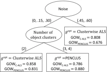
The classification tree resulting from the first step is displayed in Figure 1. It appears that for data sets with a higher amount of noise one should preferably use Clusterwise ALS. This also holds for data sets with a lower amount of noise if the true number of object clusters is small. On the other hand, for data sets with a lower amount of noise one should preferably use PENCLUS if the true number of object clusters is not too small. We may thus conclude that the most important moderators of the differential performance of Clusterwise ALS and PENCLUS are amount of noise and number of object clusters. Regarding the number of ob-ject clusters, this result may be related to the fact that PENCLUS operates in a (relaxed) continuous space while Clusterwise ALS operates in the original solu-tion space. When there is only a small number of underlying clusters, that is to say, when the original solution space is small, operating in this space appears to be better than operating in some (relaxed) continuous space. However, when there are many underlying clusters (i.e., when the original solution space is large), Clus-terwise ALS may not be moving in an efficient way throughout that space and may get lost in it. Making use of the test for disordinal interactions developed by Gail & Simon (1985), we can reject the null hypothesis of no disordinal interaction at significance levelα =.001.
Number of object clusters
𝑔opt= Clusterwise ALS
GOWC-ALS = 0.858 GOWPENCLUS = 0.831
Noise
{.45, .60} {0, .15, .30}
{2} {3, 4}
𝑔opt= Clusterwise ALS
GOWC-ALS = 0.808 GOWPENCLUS = 0.676
𝑔opt=PENCLUS
GOWC-ALS = 0.786 GOWPENCLUS = 0.880
Figure 1: Optimal data-analytic regime for the additive biclustering data resulting from the newly proposed method using classification trees. The ellipses in the figure represent the internal nodes containing the split variables, with the corresponding split point shown below each ellipse. The upper ellipsis represents the root node, which corresponds to the complete set of data sets from the benchmarking study. The rectangles represent the leaves of the tree, with each rectangle containing the assigned method, and the conditional mean outcomes under Clusterwise ALS (C-ALS) and PENCLUS.
should be specified to estimate the number of object and variable clusters in order to analyse a data set with Clusterwise ALS or PENCLUS.
To identify a proxy for the percentage of noise in the data, we relied on the object cluster membership matrix ˆAthat resulted from the ADPROCLUS analysis mentioned above with Kproxy object clusters. To obtain also a variable cluster matrix ˆBfor each data set, we subjected the transposed dataXT to ADPROCLUS, while again using the automatedCHullprocedure to select the number of variable clusters. We subsequently calculated ˆVas
ˆ
V= (AˆTAˆ)+AˆTXBˆ(BˆTBˆ)+,
with(P)+being the Moore-Penrose pseudoinverse ofP. Next, we calculated as a proxy for the percentage of noise in the data,
εproxy=||X− ˆ
AVˆBˆT||2
||X||2 ,
Proxy `Noise’
≥ .75 < .75
{2} {3, 4, 5} Proxy `Number of
object clusters’
𝑔opt= Clusterwise ALS
GOWC-ALS = 0.809 GOWPENCLUS = 0.684
𝑔opt=PENCLUS
GOWC-ALS = 0.787 GOWPENCLUS = 0.895
𝑔opt= Clusterwise ALS
GOWC-ALS = 0.835 GOWPENCLUS = 0.819
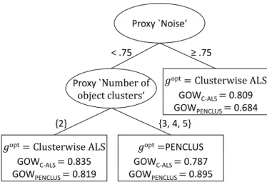
Figure 2: Optimal data-analytic regime with replacement of noise and true amount of object clus-ters by proxies that are known in data-analytic practice.
The classification tree resulting from the second analysis with the proxies for ‘amount of noise’ and ‘true number of object clusters’ as predictors is displayed in Figure 2. Interestingly, this tree has the same structure as the tree based on the originally manipulated characteristics, which gives confidence in the result and the quality of the estimated proxies. The expected outcome of the estimated optimal data-analytic regime in Figure 2 using Equation (1) is 0.844. For comparison, the expected outcome would equal 0.809 if the marginally best method, Clusterwise ALS, were applied to all 12150 data sets, and 0.788 if PENCLUS were applied to all of them. This means that, although the strategy of analyzing all data sets with Clusterwise ALS would result in an improved outcome relative to analyzing them with PENCLUS, there is added benefit to analyze them on the basis of the estimated optimal data-analytic regime.
that the optimal regime may depend on the chosen outcome measure.
A final remark pertains to the classification tree method that we used to esti-mate the data-analytic regimes in the application. Such methods are cursed by a limitation: Their search space is very large by the large number of possible split variables and the large number of possible split points per variable. This may result in instable solutions. There are several ways in which the instability of clas-sification trees can be quantified. Examples include using a bagging procedure, where a set of trees is grown based on different bootstrap samples or subsamples of the data (Breiman, 1996), and subsequently calculating a measure of instability on this set of trees (Chipman et al., 2006). A previously suggested solution for the instability problem is the use of random forests. However, a key advantage of tree-based regimes (i.e., an insightful representation of the underlying decision structure) then gets lost. An interesting potential course of action to overcome this could be to look for a precis of a random forest in terms of a single summary tree.
4. General discussion
In the present paper we introduced a novel conceptual framework and method-ology, inspired by principles of optimal treatment regime estimation, to derive op-timal data-analytic regimes from benchmarking studies with simulated data. Over and above the search of a universally winning method, this methodology provides the user with a more refined answer to questions of benchmarking in terms of how the winning method may vary over patterns of characteristics of the data and the data-generating mechanism.
In general, optimal regime estimation is fairly challenging due to the high risk of inferential errors. The underlying reason for this high risk is that (non-trivial) optimal regimes critically depend on qualitative or disordinal interactions, which imply that for some types of data, method A outperforms B, whereas for other types it is the other way around. This type of interactions is typically hard to replicate (Rothwell, 2005). The reason for this does not reside in particular methods, but in the mere fact that a reliable estimation of qualitative or disordinal interactions requires (very) large sample sizes (Lee et al., 2015). A particular ad-vantage of benchmarking studies with simulated data that may provide the basis for optimal data-analytic regime estimation is that they rather easily allow for large sample sizes, with the primary cost being computational in nature only (which in the present era of supercomputers has become less prohibitive than ever before).
hypothesis-generating devices, the results of which are to be cross-validated in replication studies. Once again such replication studies are cheaper and therefore easier to realize in the benchmarking area compared to the area of randomized clinical tri-als. Two special types of replication deserve to be singled out at this point: (a) replication studies with stratified sampling schemes, with strata corresponding to the data types identified during the optimal data-analytic regime estimation, and (b) replication studies in which variables that were not experimentally manipu-lated in the original benchmarking study (cells (c) and especially (d) of Table 1) and that appeared to be involved in the regime resulting from that study, are ex-perimentally manipulated in the follow-up replication study.
In this paper, we focused on benchmarking studies in which two methods are compared. We showed that in such cases, optimal data-analytic regimes can be estimated by using existing classification techniques that minimize some misclas-sification cost. In our case, the misclasmisclas-sification cost is data set-dependent and de-notes the loss in outcome would a data set be assigned to its non-optimal method alternative. In the illustrative application, we further focussed on methods to es-timate optimal tree-based data-analytic regimes. Typical tree-based classification techniques assume misclassification costs to be the same for all objects that are to be classified (viz., in our case, for all data sets). As a solution to work around the issue of data set-dependent costs, we made use of the fact that in quite a few tree algorithms every object can be assigned a weight. By putting these weights equal to the individual misclassification costs, application of the tree-based classifica-tion techniques in quesclassifica-tion will imply a minimizaclassifica-tion of the total misclassificaclassifica-tion cost.
tree estimation,rpart(the code of which can be obtained from the first author). The proposed method may be further extended in two ways. First, as method acts as a within-subject variable in benchmarking studies, a difference score can be used as a straightforward estimator of the contrast functionC. In optimal treat-ment regime estimation, however, the use of more involved estimators, which include an augmentation with a term borrowed from an outcome model, may be necessary (Zhang et al., 2012). It would be meaningful to explore whether a simi-lar augmentation could still further improve the quality of estimated optimal data-analytic regimes.
Secondly, we discussed the estimation of optimal data-analytic regimes on the basis of data from benchmarking studies relying on “synthetic” Monte Carlo simulations. There are no principled objections against the application of the methodology proposed in the present paper to benchmarking studies based on empirical data (which could be considered a sample from a population of data sets: Boulesteix et al., 2015). Yet, two considerable pragmatic bottlenecks need to be taken into account: (a) The sample size of benchmarking studies with em-pirical data is typically prohibitively low, and an increase of that sample size is considerably more expensive than in the case of simulated data; (b) inferences may be hampered by correlations between data characteristics across the empir-ical data sets. Taken these bottlenecks into account, a full estimation of optimal data-analytic regimes on the basis of benchmarking studies with empirical data does not look like a realistic option. As a more realistic alternative, the data sets of such studies could be used as a test bench to investigate optimal data-analytic regimes that were previously derived from benchmarking studies with simulated data sets. In case the application to the test bench would lead to unexpected dis-crepancies with the results of the simulated data sets, this could subsequently give rise to the setting up of new benchmarking studies with simulated data sets that mimic in one way or another the empirical data sets of the test bench (for an illus-tration of this principle, see Schepers et al., 2006). Otherwise, in case the primary interest of the researcher resides in outcome measures of a recovery type (as in our illustrative application), a straightforward test on empirical data is not possi-ble either. Yet, in such cases, too, one could consider to set up “realistic simulation studies” with a test bench of simulated data sets that mimic in some way empirical data sets of interest.
data-analytic regimes). Yet, the “why” of the regimes in question (i.e., the theoretical justification of why a particular method outperforms another one for certain types of data sets) should not be neglected at all. Insight into this “why” may simply lead to more sound regimes that can be extended more easily to new types of data sets.
Acknowledgements
The research reported in this paper was supported in part by the Research Fund of KU Leuven (GOA/15/003), and by the Interuniversity Attraction Poles programme financed by the Belgian government (IAP/P7/06).
References
BAIER, D., GAUL, W. and SCHADER, M. (1997). Two-mode overlapping cluster-ing with applications to simultaneous benefit segmentation and market structur-ing, inClassification and Knowledge Organization, eds. R. Klar, and K. Opitz, Berlin, Germany: Springer, pp. 557–566.
BOTH, M. and GAUL, W. (1987). Ein vergleich zweimodaler clusteranalysever-fahren.Meth. Oper. Res.57, 593–605.
BOTH, M. and GAUL, W. (1985). PENCLUS: Penalty clustering for marketing applications. Discussion Paper No. 82, Institution of Decision Theory and Op-erations Research, University of Karlsruhe.
BOULESTEIX, A.-L., HABLE, R., LAUER, S. and EUGSTER, M. J. A. (2015). A statistical framework for hypothesis testing in real data comparison studies.
Amer. Statist.69201–212.
BREIMAN, L. (1996). Bagging predictors.Machine Learning24123–140. BROOKES, S. T., WHITLEY, E., PETERS, T. J. , MULHERAN, P. A. , EGGER, M.
and DAVEY SMITH, G. (2001). Subgroup analyses in randomised controlled trials: quantifying the risks of false-positives and false-negatives.Health Tech-nol Assess51–56.
CHIPMAN, H. A., GEORGE, E. I. and MCCULLOH, R. E. (1998). Making sense of a forest of trees. In S. Weisberg (Ed.),30th Symposium on the Interface(pp 84-92). Fairfax station, VA: Interface Foundation of North-America.
DEPRIL, D. , VAN MECHELEN, I., and MIRKIN, B. G. (2008). Algorithms for additive clustering of rectangular data tables. Comput. Statist. Data Anal. 52 4923–4938.
DESARBO, W. S. (1982). GENNCLUS: New models for general nonhierarchical clustering analysis.Psychometrika47449–475.
DOOVE, L. L. , DUSSELDORP, E., and VAN MECHELEN, I. (2016).Extension
of a generic approach for estimating optimal treatment regimes to multivalued treatments.Manuscript submitted for publication.
GAIL, M. and SIMON, R. (1985). Testing for qualitative interactions between treatment effects and patient subsets.Biometrics41361–372.
GAUL, W. and SCHADER, M. (1996). A new algorithm for two-mode cluster-ing, inData Analysis and Information Systems: Statistical and Computational Approaches, eds. H.-H. Bock, and W. Polasek, Berlin, Germany: Springer, pp. 15-23.
HASTIE, T., TIBSHIRANI, R., and FRIEDMAN, J. (2009).The elements of sta-tistical learning: Data mining, inference, and prediction (2nd ed.). New York: Springer.
HOTHORN, T. and EVERITT, B. S. (2009). A Handbook of Statistical Analyses Using R (2nd ed.). Boca Raton: CRC Press.
LAGAKOS, S. W. (2006). The challenge of subgroup analyses-reporting without distorting.New England Journal of Medicine3541667–1669.
LEE, S., LEI, M.-K. and BRODY, G. H. (2015). Confidence intervals for dis-tinguishing ordinal and disordinal interactions in multiple regression.Psychol. Methods20245–258
ROTHWELL, P. M. (2005). Subgroup analysis in randomized controlled trials: Importance, indications, and interpretation.Lancet365176–186.
SHAFFER, J. (1991). Probability of directional errors with disordinal (qualitative) interaction.Psychometrika5629–38.
THERNEAU, T., ATKINSON, B. and RIPLEY, B. (2013). rpart: Recursive parti-tioning. R package version 4.1-3. http://CRAN.R-project.org/package=rpart
WILDERJANS, T. F., CEULEMANS, E. and MEERS, K. (2013a). CHull: A generic convex hull based model selection method. Behav. Res. Methods 45 1–15.
WILDERJANS, T. F., CEULEMANS, E., VAN MECHELEN, I., and DEPRIL, D. (2011). ADPROCLUS: a graphical user interface for fitting additive profile clustering models to object by variable data matrices.Behav. Res. Methods43 56–65.
WILDERJANS, T. F., DEPRIL, D. and VAN MECHELEN, I. (2013b). Additive biclustering: A comparison of one new and two existing ALS algorithms. J. Classification3056–74.
ZHANG, B., TSIATIS, A. A., DAVIDIAN, M., ZHANG, M. and LABER, E. (2012). Estimating optimal treatment regimes from a classification perspective.
Stat1103–114.
Appendix
Number of object clusters
Noise
{.30,.45, .60} {0, .15}
{2} {3, 4}
𝑔opt= Clusterwise ALS
GOWC-ALS = 0.544
GOWPENCLUS = 0.525
𝑔opt=PENCLUS
GOFC-ALS = 0.900
GOFPENCLUS = 0.915
Noise
{.15} {0}
𝑔opt= Clusterwise ALS
GOWC-ALS =0.839
GOWPENCLUS = 0.836
𝑔opt=PENCLUS
GOFC-ALS = 0.986
GOFPENCLUS = 0.990
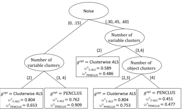
Number of variable clusters
Noise
{.30,.45, .60} {0, .15}
{2} {3, 4}
𝑔opt= Clusterwise ALS
ωA
C-ALS = 0.804
ωA
PENCLUS = 0.653
𝑔opt= PENCLUS
ωA
C-ALS = 0.762
ωA
PENCLUS = 0.909
{3,4} {2}
{2,3} {4}
𝑔opt= Clusterwise ALS
ωA
C-ALS = 0.804
ωA
PENCLUS = 0.753
𝑔opt= PENCLUS
ωA
C-ALS = 0.451
ωA
PENCLUS = 0.477
Number of variable clusters
Number of object clusters 𝑔opt= Clusterwise ALS
ωA
C-ALS = 0.589
ωA
PENCLUS = 0.486
Number of object clusters
Noise
{.30,.45, .60} {0, .15}
{2} {3, 4}
𝑔opt= Clusterwise ALS
ωB
C-ALS = 0.711
ωB
PENCLUS = 0.652
𝑔opt= PENCLUS
ωB
C-ALS = 0.762
ωB
PENCLUS = 0.906
{4} {2,3}
{.25} {.50, .75}
𝑔opt= PENCLUS
ωB
C-ALS = 0.692
ωB
PENCLUS = 0.732
𝑔opt = Clusterwise ALS
ωB
C-ALS = 0.711
ωB
PENCLUS = 0.683
Number of object clusters
Variable cluster overlap 𝑔opt= Clusterwise ALS
ωB
C-ALS = 0.625
ωB
PENCLUS = 0.546