DOI 10.1007/s10617-016-9176-2
Energy efficient semi-partitioned scheduling
for embedded multiprocessor streaming systems
Emanuele Cannella1 ·Todor P. Stefanov1
Received: 29 June 2015 / Accepted: 31 May 2016 / Published online: 16 June 2016 © The Author(s) 2016. This article is published with open access at Springerlink.com
Abstract In this paper, we study the problem of energy minimization when mapping stream-ing applications with throughput constraints to homogeneous multiprocessor systems in which voltage and frequency scaling is supported with a discrete set of operating volt-age/frequency modes. We propose a soft real-time semi-partitioned scheduling algorithm which allows an even distribution of the utilization of tasks among the available processors. In turn, this enables processors to run at a lower frequency, which yields to lower energy consumption. We show on a set of real-life applications that our semi-partitioned scheduling approach achieves significant energy savings compared to a purely partitioned scheduling approach and an existing semi-partitioned one,EDF-os, on average by 36 % (and up to 64 %) when using the lowest frequency which guarantees schedulability and is supported by the system. By using a periodic frequency switching scheme that preserves schedulability, instead of this lowest supported fixed frequency, we obtain an additional energy saving up to 18 %. Although the throughput of applications is unchanged by the proposed semi-partitioned approach, the mentioned energy savings come at the cost of increased memory requirements and latency of applications.
Keywords Energy efficient multiprocessor scheduling·Energy-efficient design·
Real-time multiprocessor scheduling·Model-based design·Embedded streaming systems
1 Introduction
Modern Multiprocessor Systems-on-Chip (MPSoCs) offer ample amount of parallelism. In recent years, we have witnessed the transition from single core to multi-core and finally to
B
Emanuele Cannella[email protected] Todor P. Stefanov
many-core MPSoCs (e.g., [13]). Exploiting the available parallelism in these modern MPSoCs to guarantee system performance is a challenging task because it requires the designer to expose the parallelism available in the application and decide how to allocate and schedule the tasks of the application on the available processors. Another challenging task is to achieve energy efficiency of these MPSoCs. Energy efficiency is a desirable feature of a system, for several reasons. For instance, in battery-powered devices, energy efficiency can guarantee longer battery life. In general, energy-efficient design decreases heat dissipation and, in turn, improves system reliability.
To address the challenge of exploiting the available parallelism and guaranteeing system performance, Models-of-Computation (MoCs) such as Synchronous Dataflow (SDF) [18] are commonly used as a parallel application specification. Then, to derive a valid assignment and scheduling of the tasks of applications, recent works (e.g., [4]) have proposed techniques that derive periodic real-time task sets from the initial application specification. This derivation allows the designer to employ scheduling algorithms from real-time theory [9] to guarantee timing constraints and temporal isolation among different tasks and different applications, using fast schedulability tests. In contrast with [4], existing techniques that exploit the analy-sis of self-timed scheduling of SDF graphs to guarantee throughput constraints (e.g., [22]) necessitate a complex design space exploration (DSE) to determine the minimum number of processors needed to schedule the applications, and the mapping of tasks to processors. Based on the analysis of [4], a promising semi-partitioned approach [7] has been proposed recently to schedule streaming applications. In semi-partitioned scheduling most tasks are assigned statically to processors, while others (usually a few) can migrate. In [7], these migrations are allowed at job boundaries only, to reduce overheads. Semi-partitioned approaches which satisfy this property are said to haverestricted migrations.
To address the energy efficiency challenge, mentioned above, many techniques to reduce energy consumption have been proposed in the past decade. These techniques exploit voltage/frequency scaling (VFS) of processors and have been applied to both streaming applications and periodic independent real-time tasks sets. VFS techniques can be either offlineoronline. Offline VFS uses parameters such as the worst-case execution time (WCET) and period of tasks to determine, at design-time, appropriate voltage/frequency modes for processors and how to switch among them, if necessary. Online VFS exploits the fact that at run-time some tasks can finish earlier than their WCET and determines, at run-time, the voltage/frequency modes to obtain further energy savings.
Problem statement To the best of our knowledge, the potential of semi-partitioned scheduling with restricted migrations together with VFS techniques to achieve lower energy consumption has not been completely explored. Therefore, in this paper, we study the problem of energy minimization when mapping streaming applications with throughput constraints using such semi-partitioned approach for homogeneous multiprocessor systems in which voltage and frequency scaling is supported with a discrete set of operating voltage/frequency modes.
1.1 Contributions
savings. In general, ourEDF-sslallows an even distribution of the utilization of tasks among the available processors. In turn, this enables processors to run at a lower frequency, which yields to lower power consumption. Moreover, compared to a purely partitioned scheduling approach, our experimental results show that our technique achieves the same application throughput with significant energy savings (up to 64 %) when applied to real-life streaming applications. These energy savings, however, come at the cost of higher memory requirements and latency of applications.
1.2 Scope of work
AssumptionsIn our work we make some assumptions that we describe and motivate below: (1) We consider systems with distributed program and data memory to ensure predictability
of the execution at run-time and scalability.
(2) We consider semi-partitioned scheduling, which is a hybrid between two extremes, par-titionedandglobalscheduling. In partitioned scheduling, tasks are statically assigned to processors. Such scheduling algorithms allow no task migration, thus have low run-time overheads, but cannot efficiently utilize the available processors due to bin-packing issues [16]. In global scheduling (e.g., [5]), tasks are allowed to migrate among proces-sors, which guarantees optimal utilization of the available processors but at the cost of higher run-time overheads and excessive memory overhead on distributed memory sys-tems. This memory overhead is introduced because in distributed memory systems the code of all tasks should be replicated on all the available cores. As shown in [7], semi-partitioning can ameliorate the bin-packing issues of partitioned scheduling without incurring the excessive overheads of global scheduling.
(3) We assume that the system’s communication infrastructure is predictable, i.e., it provides guaranteed communication latency. We include the worst-case communication latency when computing the WCET of a task. The WCET in our approach includes the worst-case time needed for the task’s computation, the worst-worst-case time needed to perform inter-task data communication on the considered platform and the worst-case overhead of the underlying scheduler as explained in Sect.2.3.
LimitationsThe problem addressed in this paper, described earlier in the problem state-ment, is extremely complex. In order to make it more tractable, our approach considers certain limitations. However, we argue that even under these limitations many hardware platforms and applications can be handled by our proposed technique. In what follows, we list the limitations considered in our proposed approach.
(1) We assume that applications are modeled as acyclic SDF graphs. Although this assump-tion limits the scope of our work, our analysis is still applicable to the majority of streaming applications. In fact, a recent work [23] has shown that around 90 % of stream-ing applications can be modeled as acyclic SDF graphs.
(2) We use a VFS technique in which the voltage/frequency mode is changed globally over the considered set of processors. Our technique, therefore, finds applicability in two kinds of hardware platforms:
– Hardware platforms that apply a single voltage/frequency mode to all the processors of the system (e.g., the OMAP 4460, as in [28]).
In the second kind of platforms listed above, our VFS technique can be used to comple-ment existing approaches that derive an efficient partitioning of tasks to clusters, such as [8,17]. Note that our proposed technique does not consider per-core VFS, therefore it may be less beneficial for systems which support this kind of VFS granularity. However, per-core VFS is deemed unlikely to be implemented in next generation of many-core systems, due to excessive hardware overhead [10].
(3) Our technique usesofflineVFS because we do not exploit the dynamic slack created at run-time by the earlier completion of some tasks. This choice is motivated by the following two reasons. (i) Online VFS may require VFS transitions for each execution of a task. Given that in our approach tasks execute periodically, with very short periods, online VFS would incur significant transitions overhead. For instance, the period of tasks in the applications that we consider can be as low as 100μs. Since the VFS transition delay overhead of modern embedded systems is in the range of tens ofμs [20], the overhead of online VFS would be substantial with such short task periods. (ii) Moreover, the existence of a global frequency for the whole voltage island renders onlineVFS less applicable. This is because online VFS would only be effective ifall cores in the voltage island have dynamic slack at the same time.
1.3 Related work
Several techniques addressing energy minimization for streaming applications have already been presented. Among these, the closest to our work are [15,22,24]. Wang et al. [24] considers applications modeled as Directed Acyclic Graphs, applies certain transformation on the initial graph and then generates task schedules using a genetic algorithm, assuming per-coreVFS. [22] assumes that applications are modeled as SDF graphs, and is composed of an offline and online VFS phases, to achieve energy optimization. As shown in Sect.3, our approach exploits results from real-time theory that allow, in the presence of stateless tasks, to set the global system frequency to the lowest value which guarantees schedulability and is supported by the system. Both [24] and [22] cannot in general make the system execute at the lowest frequency that supports schedulability because they use pure partitioned assignment of tasks to processors and non-preemptive scheduling. Finally, [15] considers both per-core and global VFS but assumes applications modeled as Homogeneous SDF graphs, and that task mapping and the static execution order of tasks is given. By contrast, our approach handles a more expressive MoC and does not assume that the initial task mapping is given.
order to reduce such overheads, while obtaining higher energy efficiency than pure partitioned approaches.
Similar to our work, other related approaches exploit task migration to achieve energy efficiency, such as [14] and [27]. In [14], the authors re-allocate tasks at run-time to reduce the fragmentation of idle times on processors. This in turn allows the system to exploit the longer idle times by switching the corresponding processors off. As explained earlier, in our approach we do not exploit run-time processor transitions to the off state because such transitions incur high overheads, especially when running dataflow tasks which have short periods.
The approach presented in [27] is closely related to ours because it leverages a semi-partitioned approach, where tasks migrate with a predictable pattern, to achieve energy efficiency. The author in [27] presents a heuristic to assign tasks to processors in order to obtain an improved load balancing. When tasks cannot entirely fit on one processor, they are split in two shares which are assigned to two different processors. Our work differs from [27] in two main aspects. First, we allow tasks with heavy utilization to be divided in more than two shares. This can yield to much higher energy savings compared to the technique proposed in [27]. Second, we allow job parallelism, i.e., we allow the concurrent execution on different processors of jobs of the same task. This, in turn, contributes to an improved balancing of the load among processors, which allows us to apply voltage and frequency scal-ing more effectively, as will be shown in Sect.3. Moreover, the applicability of the analysis proposed in [27] to task sets with data dependencies, as in our case, is questionable. In fact, the semi-partitioned scheduling algorithm underlying [27] is identical to the one proposed by Anderson et al. in [1]. As the latter paper shows, under this semi-partitioned scheduling algorithm tasks can miss deadlines by a value called tardiness, even when VFS is not consid-ered. Since in our case tasks communicate data, to guarantee that data dependencies among tasks are respected this tardiness must be analyzed. However, an analysis of task tardiness is not given by [27].
assign-ing sub-tasks load to the available processors, [19] considers onlysymmetricdistribution of the load of a task to different processors. In contrast, in our paper, as shown in Example4 in Sect.3, in order to obtain optimal energy savings we allow an asymmetric distribution of the load of certain tasks to the available processors. Second, two major differences concern the derivation of the periodic VFS switching scheme that guarantees schedulability. The first difference is that the analysis in [19] does not account for the overheads incurred when per-forming VFS transitions. By contrast, our analysis take this realistic overhead into account. The second difference is that in [19] such periodic VFS switching scheme is derived in order to meetallthe deadlines of tasks. This requires the system to perform very frequent VFS tran-sitions, especially when tasks have short periods as in our case. Conversely, in our approach we allow some task deadlines to be missed, by a bounded amount. This allows our approach to perform much fewer VFS transitions. As VFS transitions incur time and energy overhead in realistic systems, our approach guarantees higher effectiveness compared to [19].
The semi-partitioned scheduling that we propose,EDF-ssl, allows only restricted migra-tions. Notable examples of existing semi-partitioned scheduling algorithms with restricted migrations areEDF-fm[1] andEDF-os[2], from which ourEDF-sslinherits some prop-erties, as explained in Sect.2.4. The closest to ourEDF-sslisEDF-osbecause it allows migrating tasks to run on two or more processors, not strictly on two as inEDF-fm. The fundamental difference between EDF-osand our proposed EDF-ssl lays in the kind of applications that are considered by these two scheduling algorithms. InEDF-sslwe con-sider applications in which some of the tasks may be stateless and therefore can execute different jobs of the same task in parallel, if released on different processors. By contrast,
EDF-osconsiders applications modeled as sets of tasks where all tasks arestateful. This means that different jobs of the same task cannot be executed concurrently. As explained in detail in Sect.3, this fact preventsEDF-osfrom achieving energy-optimal results when streaming applications have stateless tasks with high utilization. This phenomenon is also described in the experimental results section (Sect.5.3). Similar to our work, analyses of scheduling algorithms that allow jobs within a single task to run concurrently are presented in [12,26]. However, both these works consider global scheduling algorithms which, as mentioned earlier, entail high overheads especially in distributed memory architectures. In addition, in both [12] and [26] the potential of exploiting job parallelism to achieve higher energy efficiency is not explored.
2 Background
In Sects.2.1and2.2we introduce the system model and task set model assumed in our work, respectively. Then, we summarize techniques instrumental to our approach: soft real-time scheduling of acyclic SDF graphs (Sect.2.3) and some properties of theEDF-os semi-partitioned approach which are leveraged in our work (Sect.2.4).
2.1 System model
We consider a system composed of a set= {π1, π2, . . . , πM}ofMhomogeneous
frequencies, where the maximum frequency isFN = Fmax. To ease the explanation of our
analysis, based on this maximum frequencyFmaxwe define the normalized system speed as
follows.
Definition 1 (Normalized speed)Given a frequencyFat which the system runs, this system is said to run at anormalized system speedα=F/Fmax.
This definition creates a one-to-one correspondence between any frequency at which the con-sidered system runs and its normalized speed. We will exploit this correspondence throughout this paper. Given the set of supported frequenciesΦ, by applying Definition1we obtain a set of supported normalized system speedsA= {α1, α2, . . . , αN}, whereαN =αmax=1.
2.2 Task set model
As shown in Sect.2.3below, the input application, modeled as an acyclic SDF graph with nactors, can be converted to a setΓ = {τ1, τ2, . . . , τn}ofnreal-time periodic tasks. We
assume that tasks can be preempted at any time. A periodic taskτi ∈Γis defined by a 4-tuple
τi =(Ci,Ti,Si, Δi), whereCiis the WCET of the task,Tiis the task period,Siis the start
time of the task, andΔirepresents the task tardiness bound, as defined in Definition2below.
Note thatCiis obtained at the maximum available processor frequency,Fmax. Therefore, we
can derive the worst-case task execution requirement in clock cycles asCCi =Ci·Fmax. In
this paper, we consider onlyimplicit-deadlinetasks, which have relative deadlineDi equal
to their periodTi. The utilization of a taskτiis given byu(τi)=Ci/Ti(also denoted byui).
The cumulative utilization of the task set is denoted withUΓ =τ
i∈Γu(τi).
Thekth job of taskτiis denoted byτi,k. Jobτi,kofτi, for allk∈N0, is released in the system
at the time instantri,k=Si+kTi. The absolute deadline of jobτi,kisdi,k=Si+(k+1)Ti,
which is coincident with the arrival of jobτi,k+1. We denote the actual completion time of
τi,kaszi,k. Note that the conversion of the input application to a corresponding periodic task
set, as described in Sect.2.3, creates a one-to-one correspondence between actorvi of the
application and taskτi ∈Γ. Similarly, there is a one-to-one correspondence between thekth
invocationvi,kofvi and jobτi,kofτi. These correspondences will be exploited throughout
this paper.
In this paper, we consider as soft real-time (SRT) those systems in which tasks are allowed to miss their deadline by a certain bounded value, called tardiness. The bound on tardiness is defined as follows.
Definition 2 (Tardiness bound)A task τi is said to have atardiness bound Δi ifzi,k ≤
(di,k+Δi),∀k∈N0.
Note that even if jobτi,k has tardiness greater than zero, in our approach the release time
of the next jobτi,k+1 is not affected. That is, jobτi,k+1 will be available to be scheduled
although the previous jobτi,kof taskτihas not yet finished its execution. However, in such
a case, if jobτi,kand jobτi,k+1are releasedon the same processorand the local scheduler
isEDF(as we assume in this paper) jobτi,k+1will always have to wait until the completion
of jobτi,kbecause this job has higher priority. This is because the deadline of jobτi,kis by
definition earlier than that of jobτi,k+1.
2.3 Soft real-time scheduling of SDF graphs
We define asinput actorofGan actor that receives the input stream of the application, and asoutput actorofGan actor that produces the output stream of the application. The authors in [4] show that the actors in any acyclic SDF graph can be scheduled as a set of real-time periodic tasksΓ, as defined in Sect.2.2. Their analysis begins with the computation of the WCETCi of an SDF actorvi. The value ofCi is computed such that both the worst-case
communication and computation ofvi is included:
Ci =CR·
eu∈inp(vi)
yiu+CiC+CW ·
er∈out(vi)
xir (1)
In Eq. (1),CR/CWrepresents the (platform-dependent) worst case time needed to read/write
a single token from/to an input/output channel;yiu/xir is the number of tokens read/written by actorvifrom/to edgeeu/er; inp(vi)/out(vi)is the set of input/output edges ofvi; andCiC
is the worst-case computation time of actorvi. Note thatCCi includes also the worst-case
overhead incurred by the underlying scheduler (e.g.,EDF), following the analysis of [11].
2.3.1 Derivation of minimum periods of tasks
Based on the WCETs of each actor computed by Eq. (1) and on the properties of the graph, the authors in [4] derive the minimum periodTi of each taskτi(which corresponds to SDF
actorvi ∈V), using Lemma 2 in [4]. These derived task periods ensure that each actorvi
executesqitimes in everyiteration period H:
q1T1=q2T2 = · · · =qnTn =H (2)
whereqi, derived from the properties of the SDF graph, is the number of repetitions ofvi
per graph iteration [18] andnis the number of actors in the graph.
The technique presented in [4] has been recently extended by [7], which considers that the derived periodic task set is scheduled by an SRT scheduler with bounded task tardiness (see Definition2). This extension is summarized in the following subsection.
2.3.2 Earliest start times and buffer size calculation
As long as tardiness is bounded by a valueΔi for each taskτi, earliest start times of each
taskτi can be derived (Lemma 1 in [7]). The earliest start times of taskτi corresponds to
the parameter Si defined in Sect.2.2. Similarly, minimum buffer sizes can be calculated
(Lemma 2 in [7]). Earliest start times and minimum buffer sizes are derived such that, in the resulting schedule, every actor can be released strictly periodically, without incurring any buffer underflow or overflow. Note that the technique in [7] allows tasks to miss their deadlines by a bounded value, because it uses an SRT scheduling algorithm. However, in the analysis, the worst-case tardiness that may affect each task is considered to guarantee that data-dependencies among tasks are respected. Furthermore, [7] shows that applications achieve the same throughput under SRT and HRT schedulers. In addition, even under a SRT scheduling algorithm, [7] guarantees hard real-time behavior at the interfaces between the system and the environment, provided that the buffers which implement these interfaces are appropriately sized to compensate for the tardiness of input and output actors.
Fig. 1 SDF actorsvsandvd with dependency overeu
Every invocation ofvs producesxsu tokens toeu, and every invocation ofvd consumesydu
tokens fromeu. To derive the earliest start time of the destination actorvdin presence of task
tardiness, Lemma 1 in [7] considers the worst case scheduling of the source and destination actors. This worst case scheduling, when deriving start times, occurs when the source actor vscompletes its jobsas late as possible(ALAP) and the destination actorvd is released as
soon as possible, with no tardiness. ALAP completion schedule in case of tardiness is defined below.
Definition 3 (ALAP completion schedule in case of tardiness)The ALAP completion sched-ule considers that all invocationsvi,j (jobsτi,j) of an actorvi (taskτi) incur the maximum
tardinessΔi, therefore complete atzi,k=di,k+Δi.
The ALAP completion schedule of actorvscan be represented by a fictitious actorv˜s, which
has the same period asvs, no tardiness, and start time S˜s = Ss +Δs. At run-time, any
invocation ofvs, even if delayed by the maximum allowed tardinessΔs, will never complete
later than the corresponding invocation ofv˜s. Then, the earliest start time of the destination
actorvdcan be calculated consideringv˜sas source actor.
Once the start times of source and destination actors have been calculated, Lemma 2 in [7] allows the derivation of the required size of the buffer that implements the communication overeu. Lemma 2 in [7] considers the worst case scheduling for buffer size derivation.
This occurs when the source actor executes as soon as possible, with no tardiness, and the destination actor completes its jobs as late as possible. Similarly to the analysis used to derive start times, the ALAP schedule of destination actorvdcan be represented by a fictitious actor
˜
vd which has the same period asvd, no tardiness, and start timeS˜d = Sd+Δd. Then, the
buffer size can be derived consideringvs as source actor andv˜d as destination actor.
Example 1 Consider the SDF graph shown in Fig.2a, which has three actors (v1,v2,v3) with
WCET indicated between parentheses (C1= 2,C2= 3,C3= 2) and production/consumption
rates indicated above the corresponding edges. Using Lemma 2 in [4], we derive the fol-lowing minimum periods:T1=T3= 6 andT2= 3, as shown in Fig.2b. Then, suppose that the
underlying SRT scheduling algorithm guarantees tardiness boundsΔ1= 1,Δ2= 2 (as
indi-cated in Fig.2a and shown in Fig.2b), whereasΔ3= 0. By Lemma 1 in [7], using these
tardiness bounds, we derive the earliest start timesSi shown in Fig.2b. For instance, note
thatS2= 7 ensures that any invocation ofv2will always have enough data to read as soon as
it is released. This holds even when all the invocations ofv1incur the largest tardinessΔ1,
i.e., they execute according to the ALAP completion schedule.
Note that, similar to our approach, the work in [7] also uses semi-partitioned scheduling, in which some tasks are assigned to a single core (fixed tasks) whereas some others may migrate between cores (migrating tasks). Only stateless tasks are allowed to migrate. The definition of stateless task is given below.
Definition 4 (Stateless task)A taskτiis said to be stateless when it does not keep an internal
state between two successive jobs.
(a)
(b)
Fig. 2 Example of the approach described in [7].aSimple example of an SDF graph.bDerived periodic task set and minimum start times.Up arrowsrepresent job releases, down arrows represent taskdeadlines. Only the first period ofv3is shown due to space constraints
2.4EDF-ossemi-partitioned algorithm
Our scheduling algorithm, presented in Sect.3, inherits some definitions and properties from
EDF-os[2]. Far from being a complete description of theEDF-osalgorithm, the rest of this subsection presents this “common ground” between our approach andEDF-os.
EDF-osis aimed at soft real-time systems, in which tasks may miss deadlines, but only up to a bounded value. UnderEDF-os, processors are assumed to run at the highest available frequency, which means that any processorπkcan handle a total cumulative utilization up to
1. Tasks can be eitherfixedormigrating. Migrating tasks are allowed to migrate between any number of processors, with the restriction that migration can only happen at job boundaries. Each taskτi is assigned a (potentially zero)shareof the available utilization of a processor,
as defined below.
Definition 5 (Task share)A taskτiis said to have a sharesi,konπkwhen a partsi,kof its
utilizationuiis assigned toπk.
In turn, thetask fractionof taskτion processorπkis defined as follows.
Definition 6 (Task fraction)Givensi,k,πkexecutes a fraction fi,k=sui,ik ofτi’s total
execu-tion requirement.
If taskτi is migrating, it has non-zero shares on several processors. Ifτi is fixed, it has
non-zero shares on a single processor. The share assignment inEDF-osensures that the cumulative sum of the shares of a task, over all the processors, equals the task utilization ui=
M
k=1si,k, withMbeing the total number of processors in the system.
The total share allocation on processorπkis denoted byσk
τi∈Γsi,k. In order to avoid
overloading processorπkin the long run,σk must always be lower than the total processor
utilization:
(a)
(b)
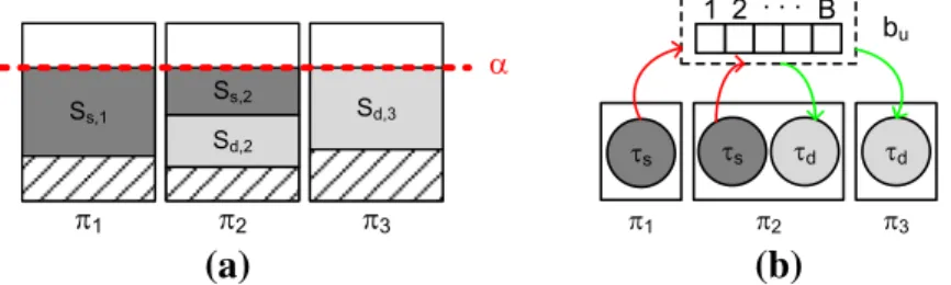
Fig. 3 Share assignments considered in Example2and Example3. Migrating tasks are indicated ingray.
aShare assignment considered in Example2.bShare assignment considered in Example3
In addition, to avoid overloading a processor in the long run,EDF-osenforces that, in the long run, the fraction of workload executed onπkis equal to the task fraction fi,kgiven by
Definition6. This long-run workload distribution according to task fractions is obtained by leveraging results from Pfair scheduling [5]. In particular, out of thefirstνconsecutive jobs released byτi,EDF-osensures that the number of jobs released on processorπkis between fi,k·νandfi,k·ν(Property 1 in [2]). Note that forν→ ∞the fraction of jobs released
onπktends to fi,k, as expected. In turn, out ofany cconsecutive jobs of a migrating taskτi,
the number of jobs released onπk(indicated asci,k) is bounded by the following expression:
ci,k≤ fi,k·c+2 (4)
The above expression is given by Property 6 in [2]. For a more detailed explanation of assignment rules for jobs of migrating tasks, the reader is referred to [1] and [2].
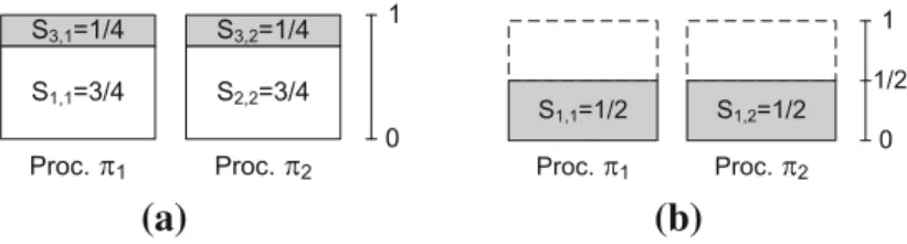
Example 2 Given the task set{τ1 = (C1 = 3,T1 = 4), τ2 = (3,4), τ3 = (1,2)}, the EDF-osalgorithm derives the task assignment shown in Fig.3a. The utilization of taskτ3in
Fig.3a is split in two shares,s3,1 = 1/4 onπ1ands3,2 = 1/4 onπ2. Therefore, in the long
run half of the jobs ofτ3will be released onπ1and the other half will be released onπ2.
3 Proposed semi-partitioned algorithm:
EDF
-
ssl
In this section we describe our proposed semi-partitioned scheduler, calledEDF-ssl. In
EDF-ssl, only stateless tasks (recall Definition4) are allowed to be migrating. We enforce this condition because migrating the internal state of a stateful task can be prohibitive in a distributed memory system. Note that underEDF-ssltask migrations can only happen at job boundaries. Once a job is released on a certain processor, it cannot migrate to another one. Moreover,EDF-sslexploits the fact that migrating tasks are stateless by allowing successive jobs to execute in parallel on different processors.
With ourEDF-sslwe want to show that, in the presence of stateless tasks, semi-partitioned scheduling can be used to improve energy efficiency, while achieving the same application throughput compared to purely partitioned scheduling. To achieve better energy efficiency it may be beneficial to run processors at voltage/frequency levels lower than the maximum. The following example shows that under certain conditions the classical partitioned VFS techniques (e.g., [3]) are not effective. Moreover, existing semi-partitioned approaches do not exploit the presence of some stateless tasks in the considered applications and therefore cannot be applied to achieve energy efficiency, if these stateless tasks have high utilization.
Example 3 Consider a single stateless taskτ1 = (C1 = 3,T1 = 3). The task utilization
(a)
(b)
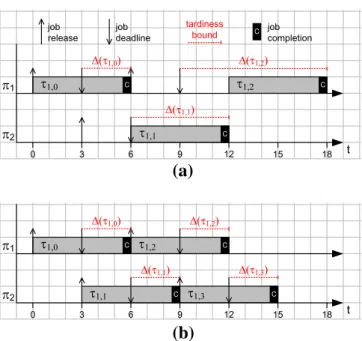
Fig. 4 Job executions ofτ1, as defined in Example3, according to the share assignment of Fig.3b.Up arrows
indicate job releases,down arrowsindicate job deadlines.Black rectanglesindicate job completion.aJob executions according toEDF-osrules.bJob executions according toEDF-sslrules
τ1 can only be assigned to one processor and this processor must run at its highest
volt-age/frequency level, becauseu1 = 1. Moreover, even existing semi-partitioned approaches
cannot distribute the utilization ofτ1over more than one processor, as shown in the
follow-ing. Assume that to improve energy efficiency the utilization ofτ1has to be split over two
cores,π1andπ2, running at half of the maximum frequency, i.e., at normalized processors
speedα=1/2. Note that under these conditions Eq. (3) has to be changed accordingly. We enforce thereforeσ1≤αandσ2≤α. The resulting assignment of shares ofτ1is shown in
Fig.3b.
In this scenario, the problem ofEDF-osis that it does not consider job parallelism. This means that jobτi,k+1 of a migrating taskτi has to wait for the completion of the previous
jobτi,k. For instance, in Fig.4a, jobτ1,0 is released onπ1at time 0. Sinceα =1/2,τ1,0
finishes at time 6. Therefore jobτ1,1, although released at time 3 onπ2, has to wait until
time 6 to start executing. As shown in Fig.4a, although jobs ofτ1are assigned alternatively
toπ1andπ2, the tardinessΔincurred by successive jobs ofτ1increases unboundedly. Our EDF-sslavoids this linkage between processors by allowing jobs released by a migrating task to execute in parallel, exploiting the fact that migrating tasks are assumed to be stateless. As depicted in Fig.4b, this leads to bounded tardiness for all jobs ofτ1.
Under ourEDF-ssl, necessary (but not sufficient) conditions to guarantee schedulability are the following. First, the total utilization of the task setΓ cannot be higher than the total available utilization on processors:UΓ ≤α·M, where Mis the number of available processors in the system and assuming that they all run at the same normalized speedα≤1. Second,αmust be greater than the utilization of any stateful task inΓ:α ≥us,max, where
us,maxis the utilization of the heaviest stateful task inΓ. This is because stateful tasks are
We merge the above two conditions in the following expression, which provides necessary higher and lower bounds forα:
max{UΓ/M,us,max} ≤α≤1 (5)
We now proceed with a detailed description of ourEDF-ssl. As in all semi-partitioned approaches (e.g., [1,2]),EDF-sslis composed of two phases, an assignment phase and an execution phase, which are described in Sects.3.1and 3.2, respectively. Tardiness bounds guaranteed underEDF-sslare derived in Sect.3.3, for the case of processors running at a fixed normalized speedα. Finally, Sect.3.4presents a processor speed switching technique, called “Pulse Width Modulation (PWM) scheme”, that provides a certain normalized speed in the long run. Tardiness bounds are derived also for the latter scenario.
3.1 Assignment phase
The assignment phase ofEDF-sslis given in Algorithm1. It consists mainly of 3 steps, which we explain below. Note that underEDF-sslprocessors can run at a normalized speedαlower than 1. Therefore, to avoid overloading processors in the long run, we modify condition (3) as follows:
σk≤α, ∀πk∈ (6)
which means that the total share assignment on any processorπkcannot exceed its
normal-ized speed. Moreover, note that executing Algorithm1makes only sense if condition (5) is satisfied.
First step (lines 1–5)In this step, the algorithm finds the set of stateful tasksΓswithin the
original task setΓ. Then, it uses the First-Fit Decreasing Heuristic (FFD) [16] to allocate these stateful tasks asfixedtasks over the available processors. This means that ifτi ∈Γs
is assigned to processorπk, its share onπk should be equal to the whole task utilization:
si,k=ui andsi,l=0,∀l=k.
Second step (lines 6–10)This step tries to assign all the remaining (stateless) tasks asfixed tasks over the remaining available processor utilization, usingFFD. The tasks which can not be assigned as fixed are added to a set of tasksΓna, which are assigned in the next step.
Third step (lines 11–17)The final step assigns all the remaining tasks, which could not be allocated as fixed tasks. Considering the processor list in reversed order{πM, πM−1, . . . π1},
taskτi ∈Γnais allocated a share on successive processors, considering the remaining
uti-lization on each processor, in a sequential order. (The remaining utiuti-lization on processorπk
is given by(α−σk)). The assignment of taskτifinishes when the sum of its shares over the
processors equals the task utilizationui. The third step considers the processor list in reversed
order as a way to minimize the number of processors, which already have fixed tasks, that are utilized to assign migrating shares. This can lead to a lower number of tasks with tardiness.
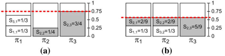
Example 4 Consider the SDF graph example in Fig.2a. In Example1, we derived the corre-sponding task setΓ = {τ1 = (2,6), τ2 = (3,3), τ3 = (2,6)}. The total utilization of the
task set isUΓ = 1/3 +1 + 1/3 = 5/3. Assume that we want to execute this task set on M=3 processors. By condition (5),α≥UΓ/M=5/9, therefore the lowestαwhich could provide schedulability isαopt=5/9. Running the system at this lowest speedαoptminimizes
the energy consumption. Now, if the system supports the speedαopt, we can simply set the
system speed to that value. In this case, we can derive tardiness bounds using the result in Sect.3.3, which considers fixed processors speed.
However, suppose that the considered system supports a set of normalized speedsA=
(a)
(b)
Fig. 5 Share assignments considered in Example4. Values ofαare shown inred.aα=0.75.bα=αopt= 5/9. (Color figure online)
Algorithm 1: Share assignment heuristic.
Input: A set ofMprocessors= {π1, π2, . . . , πM}, their normalized speedα, a set ofnperiodic tasksΓ = {τ1, τ2, . . . , τn}.
Result: AnM-partition describing the share assignment ontoMprocessors ifΓ is schedulable,False
otherwise.
FindΓs= {τ:τ∈Γ ∧τis stateful}; 1
forτi∈(Γs,sorted by decreasing utilization)do 2
Try to assignsi,k=uiof taskτion a singleπkusingFF; 3
ifFFfails for allπk∈then 4
returnFalse; 5
Γna= ∅(the set of unassigned tasks, initially empty) 6
forτi∈(Γ−Γs,sorted by decreasing utilization)do 7
Try to assignsi,k=uiof taskτionπkusingFF; 8
ifFFfails for allπk∈then 9
Γna=Γna∪τi;
10
k = M (start share assignment from processorπMtoπ1); 11
forτi∈Γnado 12
uremaining=ui; 13
whileuremaining>0do 14
si,k=min(uremaining, (α−σk)); 15
σk,uremaining=(σk+si,k), (uremaining−si,k); 16
ifσk=αthen 17
k = k-1 18
the system speed to the lowestα ∈ Asuch thatα > αopt, condition which could provide
schedulability:α =0.75. We can then refer again to Sect.3.3to derive tardiness bounds in this scenario. Fig.5a shows the share assignment of tasks inΓ, whenα = 0.75 and assuming that input and output actors (τ1,τ3) are stateful.Choice 2)We use the periodic
speed switching technique described in Sect.3.4to get the normalized speedαopt in the
long run, and we derive the corresponding tardiness bounds. Fig.5b shows the assignment obtained whenα=αopt=5/9.
3.2 Execution phase
At run-time,EDF-sslfollows the simple rules defined below.
Job releasing rulesJobs of a fixed taskτf are released periodically, everyTf, on a single
processor. Jobs of a migrating taskτm are distributed over all the processors on whichτm
migrating tasks (see Sect.2.4). In particular, Eq. (4), which provides an upper bound of the number of jobs released on a processor as a function of the migrating task share, is still valid. This result will be instrumental to the derivation of tardiness bounds under ourEDF-ssl.
Job prioritization rulesAs mentioned before, jobs of fixed and migrating tasks released on a certain processor are scheduled using a localEDFscheduler. As shown in Example3, under ourEDF-sslwhen a task migrates from a processor to another one, the job released on the latter processor does not wait until the completion of the job released on the former processor. This is in contrast with what happens underEDF-os. Moreover, contrary to our
EDF-ssl, underEDF-oscertain tasks are statically prioritized over others.
3.3 Tardiness bounds under fixed processor speed
Given the rules and properties of ourEDF-ssl, described in Sects.3.1and 3.2, we now derive its tardiness bounds, which are provided by Theorem1below. Note that due to the way task shares are assigned in the third step of the assignment phase, each processor runs at most two migrating tasks.
Theorem 1 Consider a processorπk running at a fixed normalized speedα. Assume two
migrating tasks,τiandτj, are assigned toπk. Then, jobs of fixed and migrating tasks released
onπkmay incur a tardiness of at most
Δπk = 2(Ci+Cj)
α (7)
where Ci and Cjare the worst-case execution time ofτiandτj, respectively, andαfollows
Definition1.
Proof We prove Theorem1by contradiction. We focus on a certain jobτq,l, belonging to
either a fixed or a migrating task, assigned toπk. Let assume that this job incurs a tardiness
which exceedsΔπk. We define the following time instants to assist the analysis:td is the
absolute deadline of jobτq,l;tc=td +Δπk; andt0 is the latest instant beforetcsuch that
no migrating or fixed job released beforet0 with deadline at mosttd is pending att0. By
definition oft0, just beforet0πkis either idle or executing a job with deadline later thantd.
Moreover,t0cannot be later thanrq,l, the release time of jobτq,l. Note that since we assume
that jobτq,lincurs a tardiness exceedingΔπk, it follows thatτq,ldoes not finish at or beforetc.
We denote asγ the total set of tasks, fixed and migrating, assigned toπk. We first
deter-mine the demand placed onπkbyγ in the time interval[t0,tc). By the definitions oft0,td,
andtc, any job of any task that places a demand in[t0,tc)onπkis released at or aftert0and
has a deadline at or beforetd. Therefore, the demand of any taskτiin[t0,tc)is given by the
number of jobs released in this interval multiplied by the job execution time.
The number of jobs released onπk in[t0,tc), by afixedtaskτf, is at mostc= tdT−ft0
because fixed tasks release all of their jobs onπk. By contrast, amigratingtaskτmreleases
c= td−t0
Tm jobs, but only part of them are assigned toπk. An upper bound of the amount
of jobs assigned toπk, out of everycconsecutive jobs, is given by Eq. (4).
We can now compute the total demand from tasks assigned toπk. We denote asγf and
γmthe fixed and migrating sets of tasks mapped onπk, respectively. Note thatγm= {τi, τj}.
dmd(γm,t0,tc)≤
fi,k
td−t0
Ti
+2
Ci+
fj,k
td −t0
Tj
+2
Cj
≤(td−t0)
fi,k
Ci
Ti +
fj,k
Cj
Tj
+2(Ci+Cj)
Given the definition of fi,kin Definition (6), we obtain:
dmd(γm,t0,tc)≤(td−t0)(si,k+sj,k)+2(Ci+Cj) (8)
At the same time, the demand from fixed tasks in[t0,tc)is upper bounded by:
dmd(γf,t0,tc)≤
τf∈γf
td−t0
Tf
Cf ≤(td−t0)
τf∈γf
Cf
Tf
From condition (6), we obtain:
dmd(γf,t0,tc)≤(td−t0)(α−si,k−sj,k) (9)
Combining Eq. (8) and (9), we derive an upper bound for the total demand of fixed and migrating tasks in[t0,tc):
dmd(γf ∪γm,t0,tc)≤α(td−t0)+2(Ci+Cj) (10)
To ease our analysis, we now express the total demand from tasks in clock cycles. Recall that any requirement in processor time can be converted to clock cycles. For instance, for any taskτa, its worst-case clock cycles requirement isCCa =Ca·Fmax(see Sect.2.1). Then,
from Eq. (10) we get:
dmd_cc(γf ∪γm,t0,tc)≤Fmax
α(td−t0)+2(Ci+Cj) (11)
Now, from our initial assumption that the tardiness of jobτq,lexceedsΔπk, it follows that
the amount of clock cycles provided by the processor in the interval[t0,tc)is less than the
total demand from tasksdmd_ccin the same time interval. In the considered interval, the total demand from tasks is upper bounded by Eq. (11), whereas the amount of clock cycles provided by processorπkisFmaxα(tc−t0), becauseπkruns at frequencyFmaxα. Therefore, we have:
Fmaxα(tc−t0) <Fmax
α(td−t0)+2(Ci+Cj) (12)
Dividing both sides byFmaxα:
tc<td+2(Ci+Cj)/α ⇒ tc<td+Δπk (13)
Expression (13) contradicts the earlier definition oftc = td +Δπk, therefore Theorem1
holds.
Note that the tardiness bound given by Eq. (7) differs from the tardiness bounds of EDF-osgiven by Eqs. (3) and (10) in [2]. This is caused by the differences in theexecutionphase between the two scheduling algorithm described in Sect.3.2.
3.4 Tardiness bounds under PWM scheme
The optimal normalized speedαoptwhich can minimize energy consumption while
guaran-teeing schedulability, is derived from the lower bound in expression (5). Thisαopt, however,
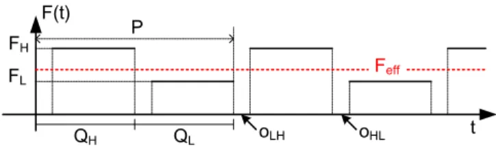
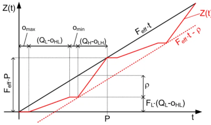
Fig. 6 PWM scheme execution
Definition1,αoptcorresponds to the optimal frequencyFoptthat can guarantee
schedulabil-ity. Although runningconstantlyat this optimal frequencyFoptmay not be supported by the
system, it is possible to achieve this optimal frequency valuein the long run, exploiting a “Pulse Width Modulation” (PWM) scheme, where the system switches periodically between two supported frequencies,FL andFH, withFL < Fopt < FH. In particular, we consider
the PWM technique presented in [6], which we summarize in the following subsection.
3.4.1 PWM scheme
The PWM scheme presented in [6] is aimed at uniprocessor systems with HRT constraints. The execution of the scheme at run-time is sketched in Fig.6. The PWM scheme switches periodically between a lower frequencyFL and a higher frequencyFH. The period of the
PWM scheme is denoted byP.
The duration of the interval of the low-frequency (high-frequency) mode isQL (QH).
Note thatQL +QH = P. Moreover, [6] definesλL = QPL andλH = QPH, the fraction of
time spent running at low and high modes, respectively.
As shown in Fig.6, the scheme considers time overheads due to frequency switching. These overheads are denoted byoLHfor transitions between lower to higher frequencies, and
byoHLfor the opposite transitions. In addition, [6] denotes the amount of clock cycles lost
during frequency transitions asΔLH=FLoHL+FHoLH.
Under the above definitions, the effective frequency obtained by running the processor at FL forQLtime andFHforQH time is given by expression (8) in [6]:
Feff=λLFL+λHFH−ΔLH/P (14)
To ensure HRT execution on the system, in their analysis the authors leverage the processor supply functionZ(t), defined as theminimum number of cycles that the processor can provide in every interval of length t. From the parameters of the PWM scheme,Z(t)is depicted with a solid red line in Fig.7, withomax=max{oLH,oHL}andomin=min{oLH,oHL}. Function
Z(t)is zero in[0,omax]; grows linearly with slope FL in[omax,omax+QL−oHL]; stays
constant in[omax+QL−oHL,omax+QL−oHL+omin]; finally, grows with slopeFHuntil
the end of the periodP. Note thatZ(t)is periodic with periodP.
3.4.2 Tardiness bounds derivation
In our approach, we leverage the processor supply functionZ(t)to derive tardiness bounds for any task running on a processor under ourEDF-sslscheduling algorithm. These tardiness bounds are given by the following theorem.
Theorem 2 Consider a processorπk, on which the PWM scheme described in Sect.3.4.1
Fig. 7 Supply functionZ(t)
WCET Ci) andτj (with WCET Cj), are assigned toπk. Then, jobs of fixed and migrating
tasks released onπkmay incur a tardiness of at most
Δπk
PWM=
2(Ci+Cj)
αeff
+ ρ
Feff
(15)
withρ=(Feff−FL)QL+FLoHL+FeffoLHandαeffis derived using Definition1from Feff.
Proof To prove Theorem2, we first derive a lower bound forZ(t). We define the following parameter:
ρ=maxt∈R+{Feff·t−Z(t)}
which represents the maximum difference between the “optimal” number of cycles, provided in[0,t]by a processor running atFeff, andZ(t). From Fig.7we get:
ρ=(Feff−FL)QL+FLoHL+FeffoLH (16)
from which we can express a lower bound forZ(t)as:
ˇ
Z(t)=Feff·t−ρ (17)
ˇ
Z(t)is depicted in Fig. 7 with a dashed red line. We can then express Z(t) as Z(t) =
ˇ
Z(t)+e(t), withe(t)≥0,∀t≥0.
Now, we follow the proof of Theorem1. This time, the instant tc is defined astc =
td+ΔπPWMk , and we assume that a certain jobτq,ldoes not complete by timetc. The definitions
oft0andtdare unchanged. The demand from fixed and migrating tasks, expressed in clock cycles, is still bounded by (11). However, we have to change the left-hand side of the inequality in (12) withZ(tc−t0), obtaining:
Feff·(tc−t0)−ρ+e(tc−t0) < Fmax
αeff(td−t0)+2(Ci+Cj) (18)
SinceFeff=Fmaxαeff, dividing both sides byFmaxαeffwe get:
(tc−t0)−ρ−
e(tc−t0)
Feff
< (td −t0)+
2(Ci+Cj)
αeff
therefore:
(tc−td) <
2(Ci+Cj)
αeff +
ρ−e(tc−t0)
Feff =Δ
πk
PWM−
e(tc−t0)
Feff
(19)
Even withe(tc−t0) = 0, which represents the worst case, expression (19) contradicts the
Note that by Eq. (15) it follows that tardiness can be experienced even on processors with no migrating tasks, given the fact that the termρdepends only on the parameters of the PWM scheme.
4 Start times and buffer sizes under
EDF
-
ssl
In Sect.2.3.2we summarize the analysis that guarantees correctness of start times and buffer sizes under the SRT scheduling algorithm used in [7], namelyEDF-fm. In order to maintain this analysis valid for our proposed EDF-ssl, we must take into account the differences between ourEDF-sslandEDF-fm.
Let us consider again the data-dependent actorsvs (source) andvd (destination) shown
in Fig.1. We recall that, as described in Sect.2.3, in our analysisvs andvd are converted
into two periodic tasksτs andτd. Assume, for instance, that the system runs at a certain
constant normalized speedα, and bothτsandτdare assigned to the processors as migrating
tasks, with the share assignment shown in Fig.8a. Sharesss,1 andss,2 ofτs are assigned
toπ1andπ2, whereas sharessd,2andsd,3 ofτd are assigned toπ2andπ3. In Fig.8a, the
dashed areas in each processor represent processor utilization assigned to tasks other than τs andτd. These other tasks are assumed to be of fixed type (i.e., not migrating). Sinceπ1
andπ3run only one migrating tasks, by Eq. (7) we derive the following tardiness bounds:
Δπ1 = 2C
s/α,Δπ2 = 2(Cs+Cd)/α,Δπ3 = 2Cd/α, whereCsandCd are the WCETs
ofτsandτd, respectively. It follows that under ourEDF-ssljobs of the same migrating task
have different tardiness bounds, depending on which processor the jobs are released. For instance, jobs ofτswill incur a tardiness of at mostΔπ2when released onπ2, andΔπ1when
released onπ1, withΔπ2 > Δπ1. By contrast, underEDF-fmused in [7], jobs of a migrating
task experience no tardiness at all, because tardiness can only be experienced by fixed tasks. In addition, under ourEDF-ssljobs of the same migrating task can execute in parallel. This cannot happen underEDF-fm.
In the remainder of this section we define a way to guarantee a correct schedule ofτs
andτd, with no buffer underflow or overflow, under ourEDF-ssl. As shown in Fig. 8b,
we assume that processors running communicating tasks have access to a shared memory where data communication buffers are allocated. Note that our approach allows data and instruction memory of all processors to be completely distributed, therefore contention can only occur when accessing the shared communication memory. In Fig.8b, bufferbuof size
Bimplements the communication over edgeeuof Fig.1. Our analysis to guarantee a correct
scheduling ofτsandτd comprises two parts. First, we guarantee valid start times ofτsand
τd and buffer size Bby adapting the analysis in [7] to ourEDF-ssl. Second, we define a
(a)
(b)
pattern thatτsandτd use when reading/writing from/tobuto ensure functional correctness.
These two parts are described below.
Part 1—Valid start times and buffer sizesAs mentioned earlier, under ourEDF-ssl
jobs of the same migrating task can have different tardiness bounds, if released on different processors. According to Definition2, the tardiness boundΔi of a certain taskτi must be
valid for all its jobs. Therefore, we set the value ofΔi to the maximum tardiness bound
among the processors which are assigned (non-zero) shares ofτi, as follows:
Δi =
maxk|si,k>0{Δπk} under fixed processor speed
maxk|si,k>0{Δ
πk
P W M} under PWM scheme
(20)
whereΔπk andΔπk
P W M are the tardiness bounds calculated for processor πk under fixed
processor speed and under the PWM scheme described in Sect.3.4.1, respectively. For each processorπk,ΔπkandΔπP W Mk are obtained using Eq. (7) and Eq. (15), respectively. Finally,
in Eq. (20)si,krepresents the share ofτionπk.
By using the tardiness bound Δi expressed by Eq. (20), we can represent the ALAP
completion schedule (see Definition3 in Sect. 2.3.2) of actor vi (corresponding to task
τi) as a fictitious actorv˜i, which has the same period asvi, no tardiness, and start time ˜
Si = Si +Δi. From Eq. (20) it follows that at run time any invocation vi,j of actor vi
will never be completed later than the corresponding invocationvi˜,j of actorv˜i, regardless
of which processor is executing that invocation. Therefore, the analysis for start times and buffer sizes in the presence of tardiness described in Sect.2.3.2can be applied considering the tardiness bounds given by Eq. (20) and it is correct for ourEDF-ssl.
Part 2—Reading/writing pattern to/frombuLet us focus on the source actorvsin Fig.1,
and let assume the share assignment shown in Fig.8a. Under ourEDF-ssl, jobs ofτs, which
correspond to invocations ofvs, may execute in parallel if released onto different processors.
Moreover, as mentioned earlier, jobs ofτsmay experience different tardiness, depending on
which processor the job is released. It follows that jobs ofτsmay write out-of-order to buffer
buin Fig.8b. This is because jobτs,k+a, for somea >0, may finish before jobτs,kif they
are released on different processors. Similarly, jobs of the destination taskτd may read from
buout-of-order.
In this scenario, it is clear thatbuis not a First-in First-out (FIFO) buffer. Thus, every job
ofτs/τd(invocation ofvs/vd) must knowwhereit has to write/read to/frombu.Part 1of our
analysis (described above) ensures that B, the size ofbu, is large enough to guarantee that
tokens produced byτswill never overwrite locations which contain tokens still not consumed
byτd. Then, givenxsu, the amount of tokens produced oneuby every job ofτs, we enforce
that job jofτs (with j ∈N0) writes tokens tobuin the order indicated by Algorithm2. In
fact, Algorithm2defines a writing pattern that follows the one which would be obtained if the jobs ofτs wrote in-order to a FIFO buffer of size Bimplemented as a circular buffer.
Lines 5-7 in Algorithm2handle the case in which thexu
s tokens are “wrapped” in the buffer.
Note that by replacing in Algorithm2xsuwithyduand write operations with read operations we obtain the reading pattern corresponding to jobjof destination taskτd.
As an example of the reading and writing pattern enforced by Algorithm2, consider the case in which the production rate of source taskτsand the consumption rate of destination
taskτd over edgeeu are the same, i.e.,xsu = ydu. In this case, job j of the destination task
τd must read tokens produced by job jof the source taskτs. This is ensured if bothτsand
τd comply to the reading/writing pattern defined by Algorithm2, regardless of theorderin
which (i) consecutive jobs ofτswrite to bufferbuand (ii) consecutive jobs ofτd read from
Algorithm 2: Write pattern of job jof source taskτs.
Input: Number of produced tokensxus, job indexj, buffer sizeB. bgn= [(xsu·j) modB] +1;
1
end=(xsu·(j+1)) modB; 2
ifbgn<endthen
3
writexus tokens frombu[bgn]tobu[end] 4
else
5
write(bgn-B+1)tokens frombu[bgn]tobu[B]; 6
writeremainingtokens frombu[1]tobu[end]; 7
5 Evaluation
In this section we evaluate the effectiveness of our semi-partitioned approach in terms of energy savings. We compare our results with the heuristic-based partitioned approach which guarantees the most balanced distribution of utilization of tasks among the available proces-sors, and therefore the least energy consumption, as shown in [3]. The authors in [3] also show that the most balanced distributions are derived when worst fit decreasing (WFD) heuristic is used to determine the assignment of tasks to processors. Each processor then schedules the tasks assigned to it using a localEDFscheduler. In the rest of this section, we will refer to this partitioned approach with the acronymPAR. Note that underPARall tasks meet their dead-lines. By contrast, our proposed semi-partitioned approach will be denoted in the rest of this section withSPwhen fixed processor speed is used, and withPWMwhen the periodic speed switching scheme is adopted. Note that although under our approach tasks may experience tardiness, this has no effect on the guaranteed throughput, which remains constant among all the considered approaches (PAR,SP,PWM). However, task tardiness has an impact on buffer sizes and start times of tasks (and, in turn, on the latency of applications), as described in Sect.4. Note that although thePARapproach provides HRT guarantees to all tasks in the system, whereas bothSPandPWMonly provide SRT guarantees, our comparison remains fair. This is because:
– As shown in [7] and mentioned in Sect.2.3.2, alsoSPandPWMcan guarantee HRT behavior at the input/output interfaces with the environment, although some of the tasks of the application may experience tardiness.
– BothSPandPWM, adopting the technique of [7] described in Sect.2.3.2, guarantee the same throughput asPAR.
These two conditions are sufficient for the kind of applications that we consider, in which throughput constraints are more relevant than application latency and memory overheads. Note also that in our scheduling framework, since actors are released strictly periodically, the application latency is the elapsed time between the start of the first firing of the input actor and the worst-case completion of the first firing of the output actor.
5.1 Power model
GHz, at a supply voltage of{0.83,1.01,1.11,1.27}V, respectively. FromΦA9we can derive
the set of supported normalized speed:
AA9= {0.292,0.583,0.767,1.0}
We use the power model of a similar dual Cortex-A9 core system, considered in [20], which we normalize to a single core:
pcpu= pdyn+psta=(0.223Vcpu2 Fcpu)+(K1Vcpu+K2) (21)
whereK1 =0.08965, K2 =0.07635,Vcpurepresents the voltage supplied to the CPU in
Volts, andFcpurepresent the CPU frequency in GHz. The model comprises dynamic power
pdynand static powerpsta, and the value ofpdynassumes that the core is fully utilized. Note
that expression (21) assumes that the processor runs at one of the supported normalized speeds αi ∈ AA9. From thisαi, we can derive the processor frequencyFcpu= Fiby Definition1.
Similarly, to a normalized speedαicorresponds an unique voltage levelVcpu. Therefore, the
power consumptionpdynandpstadepend uniquely onαi. We make this relation explicit by
using the notationpdyn(αi),psta(αi), andpcpu(αi).
5.2 Energy per iteration period
Based on the power model expressed by Eq. (21), we now proceed by deriving the energy consumption underPAR,SP, andPWM. In particular, we derive the energy consumed by the system during oneiteration period(H) of the graph (recall Eq. (2)). Note that the iteration period of the graph isthe sameandconstantamongPAR,SP, andPWM, because the periods of all tasks do not change depending on the considered scheduling approach. Note also that, regardless of the application latency, every taskτi executesqi times during one iteration
periodH(recall, again, Eq. (2)). We assume thatαis sufficient to guarantee schedulability, thereforeα ≥σk, for any active processorπk. In the following, we denote the number of
active cores withMON.
Static energy of (PAR,SP)Both these approaches run at a fixed speedαi, and the static
energy consumed in one iteration periodH is given by:
EstaH,FIX=H·pFIXsta =H·MON·psta(αi) (22)
Dynamic energy of (PAR,SP)We derive the dynamic energy consumption in one iter-ation periodH. During one iteration period, each taskτjexecutesqj = H/Tj times. Each
worst-case execution takesCj/αi time, at dynamic powerpdyn(αi). Therefore, the dynamic
energy consumed by taskτjduring one iteration periodHis:
EdynH,FIX(τj)=qj
Cj
αi
pdyn(αi) (23)
From Eq. (23) we derive the dynamic energy consumed in one iteration period H by the whole task set as follows:
EdynH,FIX= τj∈Γ
qj
Cj
αi
pdyn(αi)=
pdyn(αi)
αi
τj∈Γ
qjCj (24)
Total energy of (PAR,SP)From Eqs. (22) and (24) we derive the total energy consumed during one iteration periodH under (PAR,SP) by:
EtotH,FIX =H·MON·psta(αi)+
pdyn(αi)
αi
τj∈Γ
Total energy ofPWMUnder PWM, the system switches periodically between normalized speedsαLandαHto guarantee a certainαeffin the long run. Therefore, we cannot use Eq. (25)
to model the energy consumption per iteration period under the PWM scheme, because that expression is only valid when the system runs constantly at one of the supported normalized speedsαi. For the sake of clarity, we will denote pcpu(αL)and pcpu(αH), obtained from
Eq. (21), with pLandpH, respectively. In this scenario, the total power of a single core of
the system is provided by expression (9) in [6], reported below.
pcpuPWM=λLpL+λHpH+ESW/P (26)
whereESW =eLH−pHoLH+eHL−pLoHL, which represents the energy wasted during
two speed transitions. The termsλL,λH,oLH,oHL,P, are parameters of the PWM scheme
defined in Sect.3.4.1, whereaseLH andeHLrepresent theenergyoverhead incurred in the
speed transition fromαL toαH and vice versa. We assume thateLH = eHL = 1μJ and
oLH=oHL=10μs. These values are compatible with the findings in [20]. Now, given the
number of active coresMON, we can express the total energy per iteration periodH under PWMas:
EtotH,PWM=H·MON·pPWMcpu (27)
Note that Eq. (27) depends on Eq. (26), which in turn depends on the parameters of the PWM scheme. In particular, we have to find an appropriate value for the PWM scheme periodP. Since we assume that speed changes can only happen at the granularity of the operating system tick (which has periodTOS), we enforcePto be a multiple ofTOS. From Eq. (14),
we derive the shortest P, multiple ofTOS, that makes the overhead-induced clock cycles
loss less than =0.01 times the desiredFopt. Thus,P ≥ΔLH/(Fopt). GivenP, we find
the shortestQH, multiple ofTOS, that guarantees an effective frequencyFeffgreater than or
equal toFopt(from Eq. (14); note thatQL= P−QH). At this point, all the parameters of
the PWM scheme are known and the total energy consumption per iteration period can be derived using Eq. (27).
5.3 Experimental results
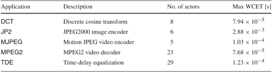
We evaluate the considered approaches (PAR,SP,PWM) on a set of real-life applications modeled as SDF graphs, which are listed in Table1. For each application, the table reports:
– a short description of its functionality (columnDescription); – the number of SDF actors (columnNo. of actors);
– the maximum WCET among actors (columnMax WCET), expressed in seconds [s].
Table 1 Characteristics of the considered applications
Application Description No. of actors Max WCET [s]
DCT Discrete cosine transform 8 7.94×10⁻⁵
JP2 JPEG2000 image encoder 6 2.88×10⁻³
MJPEG Motion JPEG video encoder 5 1.03×10⁻⁴
MPEG2 MPEG2 video decoder 23 7.68×10⁻⁵
![Fig. 2 Example of the approach described in [7]. a Simple example of an SDF graph. b Derived periodic task set and minimum start times](https://thumb-us.123doks.com/thumbv2/123dok_us/8178524.2167974/10.659.116.541.81.388/example-approach-described-simple-example-derived-periodic-minimum.webp)