Diss. ETH No. 20263
Multivariate Modelling in Non-Life
Insurance
A dissertation submitted to
ETH ZURICH
for the degree of
Doctor of Sciences
presented by
PHILIPP ARBENZ
MSc Appl. Math. ETH
born 27. March 1986
citizen of Rüti (ZH), Switzerland
accepted on the recommendation of
Prof. Dr Paul Embrechts, examiner
Dr Michel M. Dacorogna, co-examiner
Prof. Dr Giovanni Puccetti, co-examiner
Prof. Dr Mario V. Wüthrich, co-examiner
Acknowledgements
First and foremost, I am indebted to Paul Embrechts for giving me the oppor-tunity to do my PhD at RiskLab - a truly inspiring place, where ideas freely flow and swiftly flourish. His continual support and advice was invaluable.
I am most grateful to SCOR. On the one hand, SCOR provided the funds that made my PhD possible. On the other hand, SCOR allowed me to get exposed to a professional environment, where I was able to get inspired by real world problems and learn incredibly much about reinsurance.
A big thank you goes to Mario Wüthrich, Giovanni Puccetti and Michel Da-corogna for readily accepting to act as co-examiners.
During the last three years, I have been working in two worlds: ETH and SCOR. Working has been truly enjoyable in both environments. I thank my col-leagues for always being open to discussions, no matter whether the topic was a difficult mathematical proof, the relevance of stabilization clauses, or the op-timal winning strategy for the SOLA Stafette.
Therefore, many thanks for the nice time I spent at ETH go to: Daniel Alai, Peter Antal, Franziska Borer, Hans Bühlmann, Christoph Czichowsky, Matteo Casserini, Bikramjit Das, Matthias Degen, Catherine Donnelly, Vicky Fasen, Alois Gisler, Marius Hofert, Edgars Jakobsons, Dominik Lambrigger, Alex Maier, Georg Mainik, Roman Muraviev, Johanna Nešlehová, Natalia Nolde, Saša Para ¯d, Sabine Pistor, Mark Podolskij, Christian Reichlin, Annina Saluz, Andrin Schmidt, Robert Salzmann, David Stefanovits, Andreas Steiger, Augusto Teixeira, David Umbricht, Mirjana Vukelja, Sabrina Wiedersheim, David Windisch, Johanna Ziegel, Paul Ziegler, as well as the whole D-MATH Group 3.
Also many thanks to my colleagues at SCOR: Andrea Biancheri, Fabian Blatt-mann, Mathieu Cambou, Davide Canestraro, Eric Dal Moro, Raffaele Dell’Amore, Marco Demont, Allessandro Ferriero, Christoph Hummel, Stefan Küttel, An-toine Neghaiwi, Brigitte Pabst, Mladen Pavic, Nigel Riley, Jessika Walter, as well as the whole pricing, reserving and finmod teams.
Finally, I thank my family and Sandra for endless patience and constant sup-port for my mathematical and non-mathematical endeavours.
Philipp Arbenz
Abstract
A non-life insurance company is generally exposed to many risks, i.e. its con-tractual endowments generate payments in size unknown at inception date. Many of these risks have common underlying risk drivers, hence cannot be as-sumed to be independent. Multivariate stochastic models are necessary in or-der to consistently capture the joint dependence. The recent economic crisis proved (once more) that a comprehensive understanding of the dependence between and within insurance and financial risks is necessary for prudent risk aggregation. Furthermore, most regulatory frameworks such as Solvency II as well as rating agencies require such a dependence modelling. From an eco-nomic and actuarial point of view, multivariate models support making prudent risk based decisions in an insurance.
In the use of stochastic multivariate models, three steps can be identified. First, a specific model must be selected. Then the model has to be calibrated to the problem of interest. Finally, it can be evaluated with respect to quantities of interest. This thesis investigates some aspects for each of these three steps.
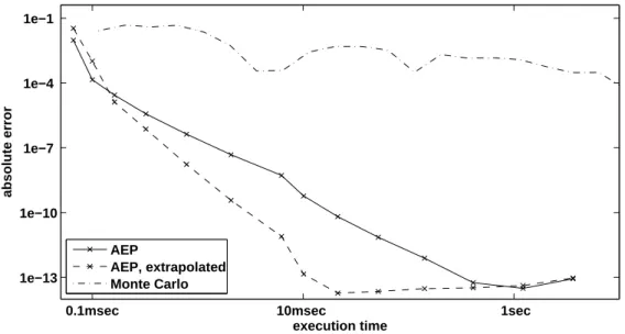
The AEP algorithm, as given in Paper A, allows to calculate numerically the distribution function of the sum of positive dependent random variables. In two to four dimensions, the AEP algorithm it is very efficient and easily outperforms Monte Carlo and Quasi Monte Carlo methods. In Paper B, the GAEP algorithm generalises the AEP algorithm for general aggregation functions.
In Paper C, we consider the estimation of a copula parameter in a Bayesian setting. Our model allows to combine different sources of information, namely observations, expert opinion and regulatory guidelines. This approach can sig-nificantly reduce the parameter estimation error when observations are scarce. Paper D introduces Hybrid Chain Ladder, a stochastic claims reserving me-thod which blends Chain Ladder and Bornhuetter-Ferguson behaviour.
In Paper E, we introduce the tree dependence model which allows to aggre-gate a very large number of risks over a hierarchical tree structure. Based on sample reordering, we give an efficient algorithm for numerical approximation. Paper F shows that the inverse Wishart distribution is not a conjugate prior to the Gaussian copula.
Kurzfassung
Nicht-Leben Versicherungen sind typischerweise vielen Risiken ausgesetzt, was bedeutet, dass sie Zahlungen erhalten und leisten deren Höhen bei Vertragsun-terzeichnung noch nicht genau bekannt sind. Viele dieser Risiken haben ge-meinsame Risikofaktoren. Daher kann man im Allgemeinen nicht annehmen, dass diese Risiken unabhängig voneinander sind. Um diese Abhängigkeiten zu erfassen sind multivariate stochastische Modelle nötig. Wie wichtig ein umfas-sendes Verständnis der Abhängigkeiten zwischen Finanz- und Versicherungs-risiken ist hat die jüngste Finanzkrise erneut gezeigt. Ausserdem verlangen so-wohl die neuen Solvenzregelungen (Solvency II, SST) als auch die Ratingagen-turen derartige Modelle. Aus aktuarieller und ökonomischer Sicht erlauben es diese Modelle in einer Versicherung risikobasierte Entscheidungen zu treffen.
Die Anwendung multivariater Modelle kann man in drei Schritte untertei-len. Zuerst muss ein mathematisches Modell ausgewählt werden. Der zweite Schritt besteht aus der Kalibrierung, beziehungsweise der Parameterschätzung. Zuletzt können Kennzahlen (Risikomasse, alloziertes Kapital, usw.) aus dem Mo-dell berechnet werden. Diese Dissertation betrachtet einige spezifische Aspekte dieser drei Schritte.
Im Paper A betrachten wir den AEP Algorithmus. Dieser Algorithmus erlaubt es, die Verteilungsfunktion einer Summe von positiven Zufallsvariablen zu be-rechnen. In Paper B wird der GAEP Algorithmus beschrieben, welcher den AEP Algorithmus auf allgemeine Aggregationsfunktionen erweitert.
Im Paper C wird die Schätzung eines Copulaparameters mit einem Bayess-chen Ansatz eingeführt. Das Modell erlaubt es, verschiedene Informationsquel-len zu vereinen, wie beispielsweise Observationen und Expertenmeinungen.
Im Paper D führen wir die Hybrid Chain Ladder Schadensreservierungsme-thode ein, welche es erlaubt für jedes Schadenjahr einen gewichteten Durch-schnitt zwischen Chain Ladder und Bornhuetter-Ferguson zu benützen.
In Paper E betrachten wir eine hierarchische Risikoaggregierungsmethode, welche es ermöglich, Abhängigkeiten in sehr hohen Dimensionen zu modellie-ren. Eine effiziente Simulationsmethode wird vorgestellt.
Paper F betrachtet einige Probleme mit konjugierten a-priori Verteilungen für Copulas, insbesondere der Gaussschen Copula.
Contents
Abstract 6
1 Introduction 13
2 Families of multivariate models 17
2.1 Hierarchical risk aggregation: the model . . . 21
3 Model calibration 25
3.1 The hybrid chain ladder method . . . 28 3.2 Estimating copulas from different sources of information . . . 31
4 Model evaluation 35
4.1 The AEP algorithm . . . 37 4.2 The GAEP algorithm . . . 43 4.3 Hierarchical risk aggregation: the reordering algorithm . . . 48
5 Conclusion 53
Accompanying papers 55
Paper A – The AEP algorithm for the fast computation of the distribu-tion of the sum of dependent random variables . . . 55 Paper B – The GAEP algorithm for the fast computation of the
distribu-tion of a funcdistribu-tion of dependent random variables . . . 89 Paper C – Estimating copulas for insurance from scarce observations,
expert opinion and prior information: a Bayesian approach. . . . 125 Paper D – On a combination of multiplicative and additive stochastic
loss reserving methods . . . 147 Paper E – Copula based hierarchical risk aggregation through sample
reordering . . . 179 Paper F – Bayesian copulae distributions, with application to
opera-tional risk management - some comments . . . 211
Cumulative Bibliography 217
Curriculum Vitae 225
12
Accompanying papers
A Philipp Arbenz, Paul Embrechts, Giovanni Puccetti.
The AEP algorithm for the fast computation of the distribution of the sum of dependent random variables.
Bernoulli17(2), 2011, 562–591.
B Philipp Arbenz, Paul Embrechts, Giovanni Puccetti.
The GAEP algorithm for the fast computation of the distribution of a func-tion of dependent random variables.
Stochastics, forthcoming in 2012.
C Philipp Arbenz, Davide Canestraro.
Estimating copulas for insurance from scarce observations, expert opinion and prior information: a Bayesian approach.
ASTIN Bulletin, forthcoming in 2012.
D Philipp Arbenz, Robert Salzmann.
On a combination of multiplicative and additive stochastic loss reserving methods.
Submitted.
E Philipp Arbenz, Christoph Hummel, Georg Mainik.
Copula based hierarchical risk aggregation through sample reordering. Submitted.
F Philipp Arbenz.
Bayesian Copulae Distributions, with Application to Operational Risk Man-agement - Some Comments.
1. Introduction
The business of an insurance or reinsurance company inherently contains many uncertainties. From a balance sheet perspective, most assets and liabilities are uncertain or risky, in the sense that amounts and timing of the correspond-ing cash flows are not known with certainty. Typical examples for such risks in a non-life insurance are: currently exposed insurance contracts, loss reserves (IBNR), assets (stocks, bonds, derivatives, etc.), reinsurance contracts, alterna-tive risk transfers, and operational risks.
The future behaviour of such risks is uncertain, as they depend on unknown future events. In most cases, one is interested in the likelihood of possible out-comes, in particular for outcomes that have an adverse economic impact. As we are interested in such likelihood, we will formulate our results in terms of prob-ability theory and we assume all random variables to be defined on a probprob-ability space (Ω,F,P).
Many of the risks to which an insurance is exposed to have common un-derlying risk drivers, i.e., their eventual future outcomes depend on the same causal factors. In this case, risks are likely to experience simultaneous posi-tive or negaposi-tive results. Hence, they cannot be assumed to be independent and their dependence structure can be seen as an effect stemming from exposure to common risk factors. One concept allowing to represent the joint distribution including the dependence structure is a multivariate model.
There are several lines of arguments supporting the claim that multivari-ate models are indeed necessary in order to prudently estimmultivari-ate, measure, and manage risks of an insurance company. We consider four perspectives: The ac-tuarial, the economic, the regulatory, and the rating agencies point of view.
From theactuarial perspective, it is important to prudently capture scenar-ios threatening solvency or even the existence of the insurance company. One important aspect is to correctly represent the likelihood of joint extreme events, i.e. the dependence structure in the joint tail of the risks. Historically, depen-dence modelling has often been ignored or was based on capturing product moment correlations. As Embrechts et al. (2002) show, models based exclusively on correlations generally have problems to adequately represent high probabil-ities of joint extreme events. Donnelly and Embrechts (2010) claim that one of
14 CHAPTER 1. INTRODUCTION
the causes of the 2008 financial crisis was the inadequate representation of tail events and their dependence. Most actuarial literature focuses on modelling de-pendencies between losses, but of course there are further relevant effects such as dependence between losses and impacts of management decisions (see Eling and Toplek (2009)) or dependence between insurance premiums and financial markets (see Jawadi et al. (2009)).
From aneconomic perspective, multivariate models form the basis of risk management. The (expected) returns of assets or liabilities must be viewed in comparison to their riskiness. The riskiness of a liability can be measured on a standalone basis or in comparison to a portfolio, which allows to take diver-sification effects into account. Such a risk assessment can only be carried out if there exists a coherent model for the joint distribution of the risks. Concepts often used in this context are capital allocation and return on risk adjusted cap-ital (RoRaC), c.f. Tasche (1999). Managing capcap-ital and its allocation in a risk ad-justed manner allows to create business incentives and constraints such that the portfolio is driven towards higher profitability, see Besson et al. (2008). Another possible positive side effect of a good risk management is the realization of tax savings through a reduction of profits’ variability. Furthermore, the presence of a sophisticated risk management usually leads to a better access to capital markets, thereby reducing refinancing costs.
From aregulatory point of view, prudent multivariate models are a way to ensure that (joint) extreme events are captured conservatively in the insurance risk management process. This protects the policy holders, who are usually the weaker parties in their relationship with the insurance company and have more difficulties to defend their interests. Through the Solvency II guidelines, Euro-pean regulators enforce the use of advanced mathematical tools to manage the risks of an insurance business. See CEIOPS (2010) and SCOR (2008) for the im-plementations of the European Union and Switzerland, respectively, as well as Dacorogna and Keller (2010) for a comparison of the two implementations. The possession of an advanced mathematical model is crucial for an insurance, but of even greater importance is that the model is fully understood, maintained, used, documented, and audited. Note that the adoption to new regulatory rules and new models often represents a big hurdle for insurance companies, in par-ticular for small companies, see Dacorogna et al. (2011), Schmitt (2011) and Fromme (2011).
15
“A. M. Best believes that enterprise risk management – establish-ing a risk-aware culture, usestablish-ing sophisticated tools to consistently identify and manage, as well as measure risk and risk correlations – is an increasingly important component of an insurer’s risk man-agement framework.”
This thesis gives an introduction to some problems related to multivariate models in a non-life insurance context. Section 2, 3, and 4 outline model selec-tion, calibraselec-tion, and evaluaselec-tion, respectively.
The subsections provide summaries of the author’s scientific contributions to the respective parts. The underlying complete papers are given in the Ap-pendix. Paper F is not summarised, as it is very short and only discusses some errors in a paper on conjugate priors for copulas.
• Section 2.1 gives an introduction to the hierarchical risk aggregation me-thod as published in Paper E. The reordering algorithm, which allows to numerically approximate the model is presented in Section 4.3.
• Section 3.1 summarises the Hybrid Chain Ladder (HCL) method proposed in Paper D. HCL is a stochastic loss reserving method which allows to blend the behaviour of Chain Ladder and Bornhuetter-Ferguson.
• Section 3.2 gives an overview on the Bayesian copula calibration method published in Paper C. It allows to combine different sources of informa-tion in order to reduce the parameter uncertainty.
• Section 4.1 gives an introduction to the AEP algorithm, which can be used to calculate the distribution function of the sum of positive dependent random variables. Paper A provides the complete underlying publication.
2. Families of multivariate models
In this section, we introduce the basic notion of multivariate models. We illus-trate three multivariate models popular in non-life insurance: variance-covari-ance approaches, risk factor models, and copula models. Section 2.1 introduces the hierarchical risk aggregation methodology published in Paper E.
LetXi:Ω→Rfor somei∈Ndenote random variables describing the
mon-etary values of losses or gains due to some risks. As a further possibility, theXi
can represent other quantitative risk characteristics, such as a natural catastro-phe (e.g. earthquake magnitude).
Suppose we are exposed to d risks: X1, . . . ,Xd. In this case, the object of
interest becomes the distribution of the random vector
(X1, . . . ,Xd) :Ω→Rd.
The stochasticity of a single riskXi is characterised through its cumulative
dis-tribution function (cdf )P[Xi ≤x],x ∈R. However, the marginal cdfsP[Xi ≤x]
do not contain any information on the dependence structure. This distribution of (X1, . . . ,Xd) is defined by its joint cumulative distribution function (cdf )
P[X1≤x1, . . . ,Xd ≤xd] , (x1, . . . ,xd)∈Rd.
This cdf contains all information on the distribution of (X1, . . . ,Xd). For
in-stance, it specifies all marginal distributions and the dependence structure. As outlined before, in many situations the components Xi cannot be
as-sumed to be independent. In this case, the joint cdf does not decouple into marginal cdfs:
P[X1≤x1, . . . ,Xd≤xd]6= d
Y
i=1
P[Xi≤xi].
A multivariate model is a model which allows to approximate the unknown true distribution P[X1≤x1, . . . ,Xd≤xd] with a distribution that captures the
important properties of (X1, . . . ,Xd). Such models are generally geared towards
simplifying the understanding, calibration, maintenance and evaluation in prac-tical problems. Of course, simplifying approaches generally contain restrictive
18 CHAPTER 2. FAMILIES OF MULTIVARIATE MODELS
mathematical assumptions, which have to be justifiable in front of management and regulator.
Many approaches for multivariate models have been proposed. Depending on the situation, different ones can be appropriate. A selection of the model should be based on the available input, the required output, and constraints such as regulatory rules:
• On the input side, we may have different sources of statistical informa-tion. With an increasing amount of data, complex models with many pa-rameters become feasible. On the other hand, parsimony should be kept in mind, as over-parametrization can lead to significant parameter risk. In some cases, the available data also contains information on the under-lying risk factors, which allows the direct modelling of those risk drivers.
• The required model output can strongly vary in an insurance context. Complicated output generally requires more sophisticated models, along with an increased complexity of estimation and evaluation. Some models may only be used to calculate the variance of a sum of risks whereas other models allow to evaluate tail risk measures of complicated aggregation functionals. Of course, it is of high relevance whether the random vector which needs to be modelled exhibits special distributional characteristics such as heavy tails, tail dependencies, or atoms. A choice of model also implies the precision with which such effects can be captured.
• Further constraints can be given by regulatory guidelines, which may spec-ify restrictions on properties or processes related to the multivariate model. For instance, the regulator can insist on models which measure the effect of parameter uncertainty on the final result.
In the following, we give a brief introduction to variance-covariance ap-proaches, risk factor models and copula models. Each of those three models has its own strengths and weaknesses. Of course, there are many more approaches for modelling multivariate risks and their dependencies, but these three are very prominent in finance and insurance, see BIS (2010) and McNeil et al. (2005).
Invariance-covariance approaches, random variables and their relation are characterised by the first two moments. Thus, for each random variable Xi,
one determines its mean µi =E[Xi] and varianceσ2i =var(Xi)< ∞. The
19
and covariance matrix
E[X]=
µ1
.. .
µd
∈Rd, cov(X)=
Σ1,1 . . . Σ1,d
..
. . .. ...
Σd,1 . . . Σd,d
∈Rd×d,
whereΣi,j=σiσjρi,j. The only constraint on the parameters is that the
covari-ance matrix cov(X) must be symmetric positive (semi-)definite. The model is “non-restrictive”, in the sense that no further assumptions are made on the dis-tribution. It is left open whether the true distribution ofX is discrete or continu-ous, and whether it has a density. No assumptions are made on higher moments (E[Xik],k>2), not even whether or not they are finite. This non-restrictiveness can be an advantage, as possibly unrealistic assumptions are avoided. On the other hand, conclusions that can be drawn from this model are inherently lim-ited to statements on the first two moments.
In arisk factor approach, one exploits the property that in many cases, the risks’ variability can be explained through a potentially low number of risk fac-tors. Risk factor models can have many different forms, but for illustrative rea-sons we concentrate on the simplest form: a linear factor model. In a linear factor model withk∈Nrisk factors, each riskXi can be written in the form
Xi=µi+ri,1Y1+ ··· +ri,kYk+ǫi.
Here,µi is the unconditional expectationµi =E[Xi]. TheYj, j =1, . . . ,k,
rep-resent the risk factors, which can be assumed to be centered (E[Yj]=0) and
normalised (var(Yj)=1) without loss of generality. The constantsri,krepresent
the sensitivity ofXi with respect to the risk factorsYk. Theǫi denote the
resid-uals, which are commonly assumed to be independent. In general, a risk factor model can be seen as a dimension reduction tool, as it allows to model a poten-tially high numberdof risks with just few risk factors (k≪d). The dependence between risks is explained by common exposure to the same risk factors.
The meaning of risk factors can be interpreted in different ways. They can represent physically observable quantities (e.g. interest rates, earthquake mag-nitudes, etc.) or they can represent an intuitively meaningless combination of variables which allow for maximal explanatory power (as done in principal com-ponent analysis).
Risk factor models can easily be generalised. For instance, the influence of risk factors can be modelled through non-linear functions. On the other hand, simplifications of the model can be attained by making restrictive assumptions on the parameters or the distribution of theǫi.
20 CHAPTER 2. FAMILIES OF MULTIVARIATE MODELS
model to estimate the distribution of the Profit-and-Loss (P&L) distribution in its Solvency II internal model, see Wilhelmy (2010).
Thecopula approachallows the full specification of the multivariate distri-bution of random vectors in terms of marginal distridistri-butions and dependence structure. The joint cdf of a random vector (X1, . . . ,Xd) can be written as
P[X1≤x1, . . . ,Xd≤xd]=C(F1(x1), . . . ,Fd(xd)) ,
where C : [0, 1]d → [0, 1] is a copula function and Fi : R→ [0, 1] denotes the
marginal cdf of Xi. A copulaC can be seen as a distribution function on [0, 1]d
with uniformly distributed margins.
Copula functions allow to separate the dependence structure from marginal distributions of a random vector. The copula determines shape and strength of the dependencies between all components of (X1, . . . ,Xd). For instance, all
rank-correlations are determined byC. On the other hand, theFi fully
deter-mines the marginal distributions of the Xi. For modelling purposes, arbitrary
models for copula and margins can be combined.
An introduction to the theory of copulas and their applications is given in Nelsen (2006) and Embrechts (2009). The separation of margins and copulas can also be seen as artificial, as discussed in the critical publication Mikosch (2006). Here, we focus on models for copulas. Different approaches and poten-tial pitfalls for marginal models in insurance can be found in Embrechts et al. (2001) and McNeil et al. (2005).
The most popular parametric copula models are elliptic copulas and Archi-medean copulas. Elliptic copulas are constructed by projecting an elliptic dis-tribution onto the unit cube by means of the probability integral transform. For an elliptic distribution with joint cdf H :Rd →[0, 1] and continuous margins, the corresponding copula is defined as
C(u1, . . . ,ud)=H
¡
H1−1(u1), . . . ,Hd−1(ud)
¢
,
whereHi−1is the inverse of thei-th marginalHi(xi)=H(∞, . . . ,∞,xi,∞, . . . ,∞).
Frequently used elliptic copulas are the Gaussian andt-copula. A generaliza-tion oft-copulas are groupedt-copulas and skewed t-copulas, see Daul et al. (2003) and Demarta and McNeil (2005).
The second class of popular copulas are the Archimedean copulas, which admit a representation
C(u1, . . . ,ud)=ψ
¡
ψ−1(u1)+ ··· +ψ−1(ud)
¢
,
2.1. HIERARCHICAL RISK AGGREGATION: THE MODEL 21
C being a copula is thatψisd-monotone. That is, thek-th derivative ofψ sat-isfies (−1)kψ(k)(x)≥0 for x ≥0 andk =0, 1, . . . ,d, see McNeil and Nešlehová (2009). The most popular Archimedean copulas are Clayton, Frank, Gumbel and Joe. These four copula classes admit a single parameter, which controls the strength of dependence. Archimedean copulas can be generalised to nested Archimedean copulas, which allow to introduce more asymmetries, see Hofert (2010b).
A third relatively popular class of copulas are the vine copulas, see Brech-mann et al. (2010). Vines split the multivariate dependence structure into pair-wise conditional dependencies, which are then modelled through bivariate cop-ulas. Vines are very flexible, but the complexity of estimation and simulation increases exponentially with the dimension.
2.1 Hierarchical risk aggregation: the model
This section gives an introduction to the hierarchical risk aggregation method-ology given in Paper E. This method allows to calculate the distribution of a sum of risks without having to specify the whole multivariate dependence struc-ture. Through the hierarchy, it suffices to specify lower dimensional depen-dence structures for each of the aggregation steps.
Suppose we are interested in the distribution of the sum
X
I∈I XI,
of random variablesXI forI in some finite set of indicesI. If theXI cannot be
assumed independent, their dependence must be modelled appropriately. As outlined above, one popular approach for dependence modelling are copulas. However, the common parametric copula models are problematic when used in high dimensions, and this for different reasons:
• The attainable dependence structures are limited and too symmetric.
• The number of parameters is inappropriate. For instance, ford margins this number tends to be too high for elliptic copulas (d(d−1)/2 parame-ters), and too low for the common Archimedean copulas (1 parameter).
22 CHAPTER 2. FAMILIES OF MULTIVARIATE MODELS
Modelling risk aggregation hierarchically can circumvent these problems. The method is intended for high dimensional applications, but for simplicity we will illustrate it with a simple three dimensional problem. The rigorous notation as well as a high dimensional example is given in Paper E.
Suppose we are interested in the distribution of the sum
X1,1+X1,2+X2
of the three random variablesX1,1,X1,2, andX2. The reason for the non-standard
index notation will become clear later. Suppose the marginal cdfs
F1,1(x)=P[X1,1≤x], F1,2(x)=P[X1,2≤x], F2(x)=P[X2≤x]
for x ∈Rare known. Assume furthermore that we are not able to model the dependence structure between those three random variables with one trivariate copula due to one of the reasons discussed above.
Instead, we conduct the risk aggregation hierarchically, in two steps:
• First, we model the dependence structure of the bivariate random vector (X1,1,X1,2) with a copulaC1: [0, 1]2→[0, 1]:
P£X1,1≤x1,X1,2≤x2 ¤
=C1 ¡
F1,1(x1),F1,2(x2) ¢
, (x1,x2)∈R2.
This defines the distribution of (X1,1,X1,2), which in turn determines the
distribution of the sub-aggregate
X1=X1,1+X1,2.
The distribution functionF1ofX1is given by
F1(t)=P[X1,1+X1,2≤t]= Z
R2
1{x1+x2≤t} dC1 ¡
F1,1(x1),F1,2(x2) ¢
fort∈R.
• Having fixed the distribution of X1, we model the copula C∅ : [0, 1]2 →
[0, 1] of the bivariate random vector (X1,X2) in the second step:
P[X1≤x1,X2≤x2]=C∅(F1(x1),F2(x2)) .
This determines the distribution of the total aggregate
X∅=X1+X2=X1,1+X1,2+X2,
as
F∅(t)=P[X1+X2≤t]=
Z
R21{x1+x2≤t} dC
2.1. HIERARCHICAL RISK AGGREGATION: THE MODEL 23
X
1,1∼
F
1,1X
∅=
X
1+
X
2∼
F
∅C
∅X
1=
X
1,1+
X
1,2∼
F
1C
1X
2∼
F
2X
1,2∼
F
1,2Figure 2.1: An illustration of the aggregation hierarchy. The three random vari-ablesX1,1,X1,2andX2have cdfsF1,1,F1,2andF2, respectively. The dependence
structures of (X1,1,X1,2) and (X1,X2)=(X1,1+X1,2,X2) are given by the bivariate
copulasC1andC∅, respectively.
This hierarchical aggregation is illustrated in Figure 2.1.
The classical copula approach for the calculation of the distribution of the aggregateX1,1+X1,2+X2would involve the determination of the trivariate
cop-ula of (X1,1,X1,2,X2). Instead, we face the task to determine two bivariate
copu-lasC1andC∅. The latter approach can be advantageous if the common
trivari-ate parametric copula families are too restrictive, too symmetric or too difficult to calibrate. Note that with the hierarchical approach, two arbitrary copulas
C1andC∅ from different copula families can be combined. Concerning
cal-ibration, it could be easier to obtain observations, expert judgement or other statistical information for (X1,1,X1,2) and (X1,X2) than for (X1,1,X1,2,X2).
The distribution ofX∅is uniquely determined. However, givenF1,1,F1,2,F2, C1, andC∅the joint distribution of (X∅,X1,X1,1,X1,2,X2) is not unique. This fact
is extensively discussed in Paper E.
The hierarchical risk aggregation can easily be extended to high dimensional problems. The model can be seen as a dimension reduction tool for the spec-ification of dependencies in a risk aggregation setting. With increasing dimen-sion, the reduction of complexity of the dependence modelling becomes more accentuated. Note that any combination of margins, copulas and aggregation hierarchy can be used.
In general, an algorithm for the generation of ani.i.d. sample of (X1,1,X1,2,X2)
heuris-24 CHAPTER 2. FAMILIES OF MULTIVARIATE MODELS
3. Model calibration
In this section, we outline some principles for the calibration of a multivariate model. Model calibration denotes the setting of parameters of the multivariate model such that the characteristics of the random vector under investigation are represented as well as possible.
In the subsections, we give brief introductions to the author’s scientific con-tributions to the topic of calibration. Section 3.1 presents the Hybrid Chain Ladder (HCL) method, which allows to estimate the distribution of outstand-ing claims based on a combination of two stochastic claims reservoutstand-ing methods. In Section 3.2, we introduce a Bayesian method for the estimation of a copula parameter, which allows to incorporate different sources of information.
Suppose a multivariate model has been selected for the modelling of the distribution of some random vector (X1, . . . ,Xd). Often, the model selection
im-plies a criterion when a model can be considered well calibrated. For instance, in a variance-covariance approach, one generally aims for a good approxima-tion of first and second moments. On the other hand, a copula model might be appropriate for the representation of tail dependencies. Having such a criterion, all available statistical information should be used to set the model parameters for an optimal fit under this criterion.
Ideally, a largei.i.d. sample {(X1i, . . . ,Xdi),i=1, . . . ,n} of (X1, . . . ,Xd) is
avail-able, which allows to calibrate the full model based on data. With increasingn, more information is contained in the sample and hence the parameter uncer-tainty can be reduced. For largen, classical statistical tools usually provide good results, see Carr and Gauger (2004) and Daykin et al. (1993). In such situations, validation tests and stresstests becomes feasible, which allows to strengthen the confidence in the model used.
In non-life insurance however, data is often very scarce or even inexistent. One reason is that many such multivariate models work on a yearly horizon and structured data gathering started only in recent years. Furthermore, many in-surance portfolios and exposures change over time, which leads to observations with differing underlying distribution.
If observations are scarce, other sources of information need to be used in order to obtain a prudent calibration. One possibility in an insurance setting are
26 CHAPTER 3. MODEL CALIBRATION
regulatory guidelines. For instance, the technical specifications of Solvency II give correlation matrices for the aggregation of many categories of risks, see Sec-tion SCR.9 in CEIOPS (2010). Similar regulaSec-tions are given in the Swiss Solvency Test, see FOPI (2006).
Another important source of relevant information is expert opinion. For in-stance, the Swiss regulator of insurances explicitly considers expert judgement for model parameter estimation, see FINMA (2008). Although expert opinion is inherently subjective, the decisions based on it are to be taken in a ratio-nal manner and should be perceived as such. To that end, many guidelines and procedural proposals have been proposed. For instance, experts need to be selected appropriately, see Cooke and Goossens (2000b). Furthermore, ac-cording to Cooke (1991), elicitation procedures need to be set such that re-producibility, fairness, accountability, and neutrality are guaranteed. Even if procedures are well designed, experts are usually still susceptible to mislead-ing psychological effects when assessmislead-ing probabilistic quantities, see O’Hagan et al. (2006) and Kynn (2008). As an illustration, consider the example given in Eddy (1982): doctors are likely to confuse P[positive test|disease] (i.e. the test sensitivity) withP[disease|positive test] (i.e. the power of the test). Further psy-chological and procedural principles which help turning expert opinion into scientifically meaningful statements are given in Meyer and Booker (2001) and Ouchi (2004).
In an insurance context, it often happens that the properties of marginal risks are already predetermined. This can be the case if there are standard me-thodologies for the estimation of marginal distributions of some risk types, but none for the joint distribution. The estimated marginal distribution may be given in different forms, such as simulations (e.g. for bootstrapping reserving methods and simulation tools for natural catastrophes), parametric distribu-tions (e.g. analytic frequency severity loss models), indirectly through moment estimates (e.g. distribution free loss reserving methods), or posterior parame-ter distributions in Bayesian models (e.g. credibility models). In this case, the multivariate model must be enforced to conform with the predetermined mar-gins. This leaves open the calibration of the dependence structure between the margins.
In the following, we describe some aspects of the calibration of the three models introduced in Section 2: variance-covariance approaches, risk factor models and copula models.
In avariance-covariance approach, no distributional assumptions are made on the joint distribution of (X1, . . . ,Xd). Therefore, non-parametric empirical
27
For a sample {(X1k, . . . ,Xdk),k=1, . . . ,n} unbiased estimators are
b
µi=
1
n
n
X
k=1
Xk, Σbi,j=
1
n−1
n
X
k=1 ³
Xik−µbi
´³
Xkj −µbj
´
.
Alternative deductions lead to different normalizations of the covariance esti-mate. For instance, the minimum mean squared error estimator uses 1/(n+1) instead of 1/(n−1).
These estimators above are not robust, i.e., they are very sensitive to out-liers. One possibility to circumvent this problem is trimming or Winsorising, which changes weight or value of extremes in the sample. An even more robust estimation method is to setµbi andΣbi,j according to median and interquartile
ranges, see Huber and Ronchetti (2009).
In arisk factor model, as outlined in Section 2, calibrating the model means finding the risk factorsYj and estimating the parametersµi, ri,j andσ2i. The
dependence between theXi is controlled by theri,j andσ2i.
For many types of insurance risks, the underlying risk factors are inherent. For instance, most claims in agriculture insurance are caused by drought, flood and hail. The elicitation of such lists of risk factors usually involves expert judge-ment and, as stated before, requires the adherence to expert elicitation guide-lines. In financial applications, often a large amount of data is available, in which case, one can also statistically find risk factors through principal com-ponent analysis.
Having determined the risk factors, one can proceed with estimating the parametersµi, ri,j andσ2i. With enough observations, these can be estimated
through regression. Depending on the amount of available information, one can also employ simplifying assumptions as outlined in Section 2. If distribu-tional assumptions are made for theXi andǫi, maximum likelihood can also be
applied. If observations are scarce, which is frequently true in insurance, one again has to resort to expert judgement. In this case, the calibration can be-come very difficult, in particular if the number of risks and risk factors is large.
The calibration of acopula modelcan generally be split into two parts. First, the distributions of the margins need to be set. Secondly, the dependence struc-ture (i.e. copula) between the margins has to be calibrated.
es-28 CHAPTER 3. MODEL CALIBRATION
timated and then the copula parameters are set accordingly. In insurance, in-formation or observations on the joint distribution of risks can be very scarce, even if there is plenty of information on the margins. Lack of data may strongly impede a prudent estimation of dependence models.
There are many statistical techniques to estimate copulas: parametric (see McNeil et al. (2005)), non-parametric (see Genest et al. (2009b), Lowin (2011) and Sancetta and Satchell (2004)) as well as Bayesian (e.g. Paper C). In high dimensions, many of these techniques become problematic, in the sense that they are computationally challenging, see Hofert (2010a).
3.1 The hybrid chain ladder method
The Chain-Ladder (CL) and Bornhuetter-Ferguson (BF) methods are standard methods in claims reserving. There is a vast amount of literature about differ-ent approaches that allow to embed the CL and BF methods within a stochastic framework. These stochastic models usually induce predictors of the ultimate claims as well as estimates of the prediction error (MSEP) and the uncertainty in the claims development result (CDR). It is common practice for reserving actu-aries to consider the results of both CL and BF and then decide for each accident year separately whether CL reserves or BF reserves are used. However, when working in a distribution-free environment, such an approach leads to mathe-matical inconsistencies, as the underlying assumptions of CL and BF are incom-patible. In this section, we introduce the hybrid chain ladder (HCL) method, which solves the problem of conflicting assumptions. It allows to set reserves for each accident year separately as a weighted average of two approaches, where the first resembles CL, and the second behaves like BF. Details and precise math-ematical deductions are given in Paper D.
Let us first introduce some notation. Let theCi,j denote the cumulative
claims of accident year i =1, . . . ,I after development year j =0, . . . ,J with J ≤ I−1. Moreover, denote byDI =©Ci,j : 1≤i≤I, 0≤j≤J,i+j≤Iª the
trape-zoid of observations up to the I-th accounting year, illustrated in Figure 3.1. Stochastic reserving methods aim to predict the yet unknown lower triangle
Ci,j ∉DI, i.e. the outstanding liabilities. In particular, we are interested in the
prediction of the ultimate claimCi,J for each accident year.
We briefly summarise the main aspects of CL and BF with respect to claims prediction. CL predictsCi,J by
b
CiC L,J =Ci,I−ifbI−i+1···fbJ,
where the fbj are estimators of the age-to-age factorsfj. These factors indicate
3.1. THE HYBRID CHAIN LADDER METHOD 29
Ci
,
J
ul
ti
m
ate
c
laims
1 j J
I i
DI
ac
cident
y
ear
i
1
2
to be predicted 2
0
observations ofCi,j
development yearj
. . . . . .
3 .. .
.. .
Figure 3.1: The trapezoidDI of cumulative claims known in accounting yearI.
The lower right triangle is yet unknown and has to be predicted.
one development year to the next development year. On the other hand, BF predictsCi,J by
b
CiB F,J =Ci,I−i+µi(γbI−i+1+ ··· +γbJ),
where theµiis a prior estimate ofCi,J and theγbjare estimates of the fraction of
claims expected in development year j. The CL predictorCbC Li,J depends multi-plicatively onCi,I−i, whereas the BF predictor has an additive structure.
There-fore, in the the CL model fluctuations on the diagonal have a much larger impact on the predicted ultimate than for BF. Although the BF method is more robust with respect to such fluctuations, it needs additional information from experts, which comprises an additional source of uncertainty.
In practice, one frequently encounters claims reserving triangles in which CL is appropriate for some accident years, whereas BF is suitable for the oth-ers. One possible cause, as stated by Neuhaus (1992), is data sparsity: trian-gles with missing entries or zero cumulatives for recent accident years. Fur-thermore, reserving actuaries often have additional external knowledge on the causes of fluctuations in the triangle. For instance, an actuary may classify a cer-tain value on the diagonal as an outlier, whose effect on the final reserves would be amplified by a multiplicative reserving method like CL. Thus, such external knowledge gives the actuary the possibility to determine for each accident year whether a multiplicative reserving behaviour (as in CL) or an additive behaviour (as in BF) is more appropriate.
30 CHAPTER 3. MODEL CALIBRATION
working in the distribution-free setting given in Mack (1993) and Mack (2008b). One inconsistency is the dependence between different increments: In BF, in-crements are independent, whereas consecutive inin-crements are dependent in CL. As these assumptions are applied to the whole triangle when estimating pa-rameters, one simultaneously imposes an incompatible set of assumptions on the triangle.
Reserving models that allow for a combination of CL-style and BF-style re-serves have already been studied in the literature. A credibility approach is given by the Benktander-Hovinen method, see Benktander (1976). In Neuhaus (1992) and Mack (2000) this credibility mixture of CL and BF is further studied but they do not specify a concrete parametric model and do not deduce a parameter es-timation error. Alai (2010) provides a solution within a generalised linear model (GLM) framework. Bayesian approaches are proposed in Verrall (2004) and Sec-tion 4.3.2 of Wüthrich and Merz (2008), respectively.
The HCL reserving method is designed to circumvent the mentioned breach of assumptions within a distribution-free setting. It allows the reserving actuary to choose for each accident year whether the reserves are determined through a multiplicative or an additive approach.
Letγj for j =0, 1, . . . ,J denote the incremental claims pattern, i.e. the
frac-tion of claims expected in development year j. The main characteristic of CL is that reserves are estimated by scaling the last known claim amount with an appropriate factor. In terms of theγj, a CL-like behaviour is then obtained by
assuming the claims process (Ci,0,Ci,1, . . . ,Ci,J) for each accident yeari =1, . . . ,I
to satisfy
E[Ci,j|Ci,j−1]=
γ0+ ··· +γj
γ0+ ··· +γj−1 Ci,j−1.
On the other hand, BF estimates reserves through an appropriate share of a prior estimate of the ultimate claims. Therefore, a BF-like behaviour of the claims process is obtained by assuming
E[Ci,j|Ci,j−1]=Ci,j−1+µiγj.
Letβj the cumulative pattern, i.e.,βj =Pij=0γjand note that (γ0+···+γj)/(γ0+
··· +γj−1)=1+γj/βj−1. The main idea of the HCL method is to take a mixture
of the above expressions:
E[Ci,j|Ci,j−1]=αi,j
µ Ci,j−1
µ
1+ γj
βj−1
¶¶
+(1−αi,j)
¡
Ci,j−1+µiγj
¢
=Ci,j−1+γj
µ
αi,j
Ci,j−1
βj−1 +
(1−αi,j)µi
3.2. ESTIMATING COPULAS FROM DIFFERENT SOURCES 31
where theαi,j∈[0, 1]. Theαi,jare weights which determine whether the claims
process behaves rather in a multiplicative behaviour (forαi,j≈1) or rather in an
additive fashion (forαi,j ≈0). The reserving actuary can set theαi,j according
to his (external) knowledge, differently for each accident and development year. Under these assumptions, it is easy to show that the expectation of the ulti-mateCi,J given the last diagonal valueCi,I−i is equal to
E[Ci,J|Ci,I−i]=Ci,I−i
Y
I−i<m≤J
ξi,m+µi
X
I−i<n≤J
Ã
(1−αi,n)γn
Y
n<m≤J
ξi,m
!
,
whereξi,j=1+αi,jγj/βj−1. In the extreme cases, where allαi,j=1 orαi,j =0,
the above expression forE[Ci,J|Ci,I−i] can be rewritten as
E[Ci,J|Ci,I−i]=
Ci,I−i Q I−i<j≤J
βj−1+γj
βj−1 , ifαi,j=1, forj=I−i+1, . . . ,J, Ci,I−i+µi P
I−i<j≤J
γj, ifαi,j=0, forj=I−i+1, . . . ,J.
In paper D, we show how parameters can be estimated, such that the ulti-matesCi,J can be predicted. This is done in a framework very close to the
clas-sical Mack approach Mack (1993). We also give methodologies to estimate the prediction error (MSEP) and the uncertainty in the claims development result (CDR). An implementation of the method in an Excel spreadsheet is available at
✇✇✇✳❘✐s❦▲❛❜✳❝❤✴❤❝❧♠❡t❤♦❞.
In future research, we propose to investigate the differences in terms of re-serves, MSEP and CDR between HCL and other proposals to combine CL and BF, such as Alai (2010) and Verrall (2004).
3.2 Estimating copulas from different sources of
information
In insurance, it is crucial to take into account the effects of dependence when modelling the joint distribution of risks. Estimating the dependence structure is relatively easy if many joint observations are available, see McNeil et al. (2005). However, in a (re)insurance setting, often only fewjointobservations are avail-able, which may be the case even if plenty of information is available for the marginal distributions. This section provides a brief introduction to the cop-ula estimation model given in Paper C. It allows to estimate a copcop-ula parameter based on different sources of information, which can reduce the parameter es-timation uncertainty.
32 CHAPTER 3. MODEL CALIBRATION
the dependence structure of a bivariate random vector (X1,X2) through a
cop-ulaC: [0, 1]2→[0, 1], i.e.,
P[X1≤x1,X2≤x2]=C(F1(x1),F2(x2)) .
Furthermore, we make the following assumptions:
• A dependence measureρ(·,·) is given, i.e. a functional measuring the de-gree of dependence between two random variables. We assume thatρis independent of the margins.
• The marginal distributionsF1andF2are continuous and known.
• The copulaC is contained in a familyC ={Cθ:θ∈Θ} of absolutely
con-tinuous bivariate copulasCθ : [0, 1]2 →[0, 1], parametrised through the
dependence measureρ, meaning thatP[U1≤u1,U2≤u2]=Cθ(u1,u2)
im-pliesρ(U1,U2)=θ.
Examples for dependence measures which are independent of marginal distri-butions are Kendall’s tau and asymptotic tail dependence. Most popular para-metric copula models can be parametrised in terms of a dependence measure
ρ.
With the assumptions above, estimating the dependence structure of (X1,X2)
is equivalent to the estimation of the parameterθ=ρ(X1,X2). If many
observa-tions are available, the standard tools from statistics can be used, such as max-imum likelihood or method of moments. However, if observations are scarce, these methods are not stable and the estimation error can become large. The actuary may choose to use also other sources of information in order to get a more robust parameter estimate. To that end, we assume the following three sources of information to be given:
1. A setE ofNindependent observations (X1,n,X2,n),n=1, . . . ,N, of (X1,X2);
2. FromKexperts, a setOof point estimatesϕkofρ(X1,X2),k=1, . . . ,K; and
3. An additional prior source of information (e.g. a regulatory guideline) which provides an estimate ofρ(X1,X2).
3.2. ESTIMATING COPULAS FROM DIFFERENT SOURCES 33
Proposition 3.1 Suppose
1. Conditionally on the degree of dependence θ, (X1,X2) has a distribution given by the copula C=Cθ∈C.
2. Conditionally on θ, the expert point estimatesϕk are independent with conditional density gk(ϕk|θ).
3. Conditionally onθ,E andOare independent.
4. The prior source of information can be translated into a prior density p(θ). Then the posterior density p(θ|E,O)ofθgivenE andO satisfies
p(θ|E,O)∝p(θ)
N
Y
n=1
c¡F1(X1,n),F2(X2,n)
¯
¯θ¢
K
Y
k=1
gk(ϕk|θ),
where c(·|θ)denotes the density of Cθ(·,·)and the symbol∝denotes
proportion-ality with respect toθ.
The proof follows from Bayes’ Theorem and is given in Paper C. Any Bayesian point estimator can now be used to calculate a point estimateθbof the copula parameter fromp(θ|E,O). We propose to use the posterior meanE[θ|E,O]. An
example illustrating the use of Proposition 3.1 is given in Paper C.
In an insurance context, it is important to guarantee a reliable and robust expert judgement process which is credible in the view of insurance, regulator and rating agencies. Decisions must be taken in a rational manner and have to be perceived as such. To that end, it is necessary to follow certain psychological and procedural principles to turn expert opinion into scientifically meaningful statements. For an overview of the literature on the use of expert opinion we refer to Meyer and Booker (2001), Ouchi (2004) or Cooke (1991). In Paper C, we give some illustrative examples for psychological pitfalls. The direct elicitation of the value of the canonical copula parameter is not feasible as this quantity may not be familiar to the expert in terms of the way he collects and evokes his knowledge. However, a question that asks for the value of a dependence measure can be formulated in a way such that substantial answers can be given even if experts are unfamiliar with probability theory.
34 CHAPTER 3. MODEL CALIBRATION
4. Model evaluation
In this section, we discuss applications of multivariate models in an insurance context. We illustrate such model evaluations based on variance-covariance, risk factor, and copula approaches. In the subsections, we summarise the au-thor’s scientific contribution to the topic of numerical model evaluation. In Sec-tion 4.1, the AEP algorithm is illustrated. The GAEP algorithm, a generalizaSec-tion of AEP, is introduced in Section 4.2. In Section 4.3, we give a method for the nu-merical approximation of the hierarchical risk aggregation model introduced in Section 2.1.
Suppose we have selected a specific multivariate model for the risks of the insurance company of interest according to the procedures outlined in Sec-tion 2. Furthermore, assume the model has been calibrated as illustrated in Section 3. The following list gives possible applications, most of them very rele-vant for the business of an insurance company.
• In many cases, the most important model application isrisk aggregation. That is, the calculation of the distribution of the sum of all risks, or of some non-linear aggregation functional. Diversification effects can usually also be assessed through the risk aggregation methodology.
• Strongly reliant on risk aggregation is the calculation ofsolvency capital requirements, which is often measured by applying a risk measure to the sum of all risks. For instance, such requirements are mandated by the European Solvency II framework or the Swiss Solvency Test.
• An involved multivariate risk model can also cover market risk factors, such as interest rates, currencies, and inflation. Knowing the sensitivity of single and aggregated insurance risks with respect to these market risks allows forasset liability management, risk hedging, duration matching, and calculation of replicating portfolios. The investment strategy should take these sensitivities into account in order to manage risk exposures.
• Knowing the joint distribution of single risks and the aggregated risk al-lows forcapital allocation, i.e. the splitting of risk capital to single risks
36 CHAPTER 4. MODEL EVALUATION
or risk classes. Through capital allocation and associated hurdle rates, portfolios can be steered towards profitability, see Besson et al. (2008). A related profitability measurement concept is RoRaC (Return on Risk ad-justed Capital).
• Having a precise multivariate model for insurance risks allows to identify the risks which constitute the major threats for the profitability or even existence of a reinsurance company. Throughreinsurance optimization
or insurance linked securities such threats can be mitigated.
We now illustrate how the tasks listed above can be solved for variance-covariance, risk factor, and copula approaches.
The conclusions that can be drawn from a variance-covariance approach
are inherently limited to mean, variance and covariance of linear combinations of the risksX1, . . . ,Xd. For instance, the characteristics of the aggregate riskS=
X1+ ··· +Xd are given by
E[S]=µ1+ ··· +µd and var(S)= d
X
i=1
d
X
j=1
cov(Xi,Xj)= d
X
i=1
d
X
j=1
σiσjρi,j.
As the model assumptions are restricted to first and second moments, no fur-ther properties ofScan be deduced. Therefore, the only sensible approach to determine risk capital in this model is to set it proportional to variance or stan-dard deviation of S. Capital can be allocated to the single risks by calculating the single risk’s contribution to the aggregate in terms of the covariance
cov(Xi,S)= d
X
j=1
cov(Xi,Xj)= d
X
j=1 Σi,j.
Portfolio optimization can be done by minimizing the variance under constraints on the portfolio decomposition. Finding optimal reinsurance strategies is anal-ogous if only proportional reinsurance contracts are considered.
In a risk factor model, Monte Carlo simulations are usually employed for model evaluation purposes. Suppose the distribution of theYj andǫi, as well
as the parametersµi,ri,j andσ2i are known, or estimated as illustrated in
Sec-tion 3. A sample of the random vector (X1, . . . ,Xd) can now easily be created by
simulating the risk factorsYj and the residualsǫi. If there is sufficient amount
of observations, one may also draw fromYj andǫi through bootstrapping. The
empirical distribution obtained through the simulations can now be used to es-timate functionals of (X1, . . . ,Xd).
4.1. THE AEP ALGORITHM 37
given by a copula model
P[X1≤x1, . . . ,Xd≤xd]=C(F1(x1), . . . ,Fd(xd)) ,
where both copula and margins are known or estimated. Realizations of (X1, . . . ,Xd)
can be generated as follows by drawing first a sample of from the copula:
¡
U1k, . . . ,Udk¢∼C, for k=1, . . . ,n. Then, a sample of (X1, . . . ,Xd) is given by
¡
X1k, . . . ,Xdk¢=¡F1−1(U1k), . . . ,Fd−1(Udk)¢, for k=1, . . . ,n,
whereFi−1is the generalised inverse ofFi. As soon as this sample is obtained,
evaluating the problems as mentioned in the beginning of this section is rela-tively easy, by using the empirical distribution of (X1, . . . ,Xd).
However, both steps of the sampling procedure for (X1, . . . ,Xd) can be
nu-merically challenging. Some parametric copula families are easy to simulate from, for instance the Gaussian copula and most Archimedean copulas, see McNeil et al. (2005). Other copula families, such as nested Archimedean cop-ulas and vine copcop-ulas require difficult numerical procedures for sampling, see Hofert (2010b) and Kurowicka and Cooke (2006). Inverting the marginal cdfs can also be non-trivial, such as in the case of stable distributions, see Hofert (2012).
4.1 The AEP algorithm
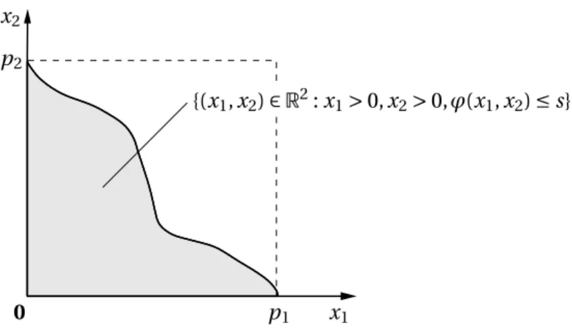
In this section, we introduce the AEP algorithm, as published in Paper A. Sup-pose we are interested in the cdf ofS=X1+ ··· +Xd, the sum of positive
depen-dent random variablesXi, at some fixed points∈[0,∞):
P[X1+ ··· +Xd≤s]. (4.1)
The AEP algorithm is designed to approximate (4.1). This algorithm does neither rely on simulations (as Monte Carlo) nor on numerically integrating a density. Instead, it approximates (4.1) through a geometric approach, using only evaluations of the joint cdf of (X1, . . . ,Xd).
The two necessary assumptions for its application are that
• all components of the random vector X = (X1, . . . ,Xd) are positive, i.e.
P[Xi>0]=1 fori=1, . . . ,d,
• the joint cdf
H(x1, . . . ,xd)=P[X1≤x1, . . . ,Xd ≤xd]
38 CHAPTER 4. MODEL EVALUATION
The first assumption can be weakened to component-wise bounded from be-low. The second assumption is satisfied, for instance, if the distribution of X
is given through a copula model where both copula and marginal distribution functions are analytic.
Here, we give an overview on the most important aspects of the AEP algo-rithm. To that end, we concentrate on the graphically intuitive two dimensional cased=2. The general cased∈Nis given in Paper A.
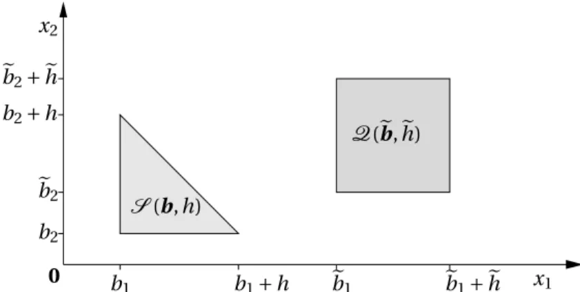
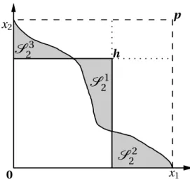
First, we give some definitions. Forb=(b1,b2)∈R2andh∈R,Q(b,h)⊂R2
denotes the hypercube
Q(b,h)=
(
(b1,b1+h]×(b2,b2+h] ifh>0,
(b1+h,b1]×(b2+h,b2] ifh<0.
LetVH denote the (probability) measure onR2induced by the joint cdfH
VH[(−∞,x1]×(−∞,x2]]=H(x1,x2).
The probability P[(X1,X2)∈Q(b,h)]=VH[Q(b,h)] forh>0 can easily be
ex-pressed in terms ofH:
VH[Q(b,h)]=P[X ∈(b1,b1+h]×(b2,b2+h]]
=H(b1+h,b2+h)−H(b1,b2+h)−H(b1+h,b2)+H(b1,b2). (4.2)
The caseh<0 is analogous.
LetS(b,h)⊂R2denote the simplex
S(b,h)=
(©
x∈R2:x1−b1>0,x2−b2>0, andP2k=1(xk−bk)≤h
ª
if h>0,
©
x∈R2:x1−b1≤0,x2−b2≤0, andP2k=1(xk−bk)>h
ª
if h<0.
The definitions of the setsQ(b,h) andS(b,h) are illustrated in Figure 4.1.
Recall that we intend to calculate or approximateP[X1+X2≤s]. In terms of
the probability measureVH,P[X1+X2≤s] can be written as P[X1+X2≤s]=VH[S(0,s)] .
Due to (4.2), it is very easy to compute theVH-measure of squares. The idea
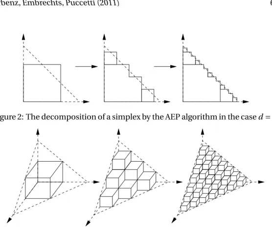
behind the AEP algorithm is to approximate the simplexS(0,s) by squares and
through the probability mass of these squares approximateP[X1+X2≤s].
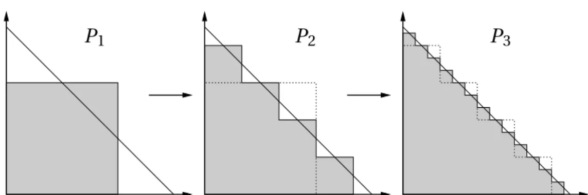
As a first proxy toS1
1 =S(0,s), we set
Q1
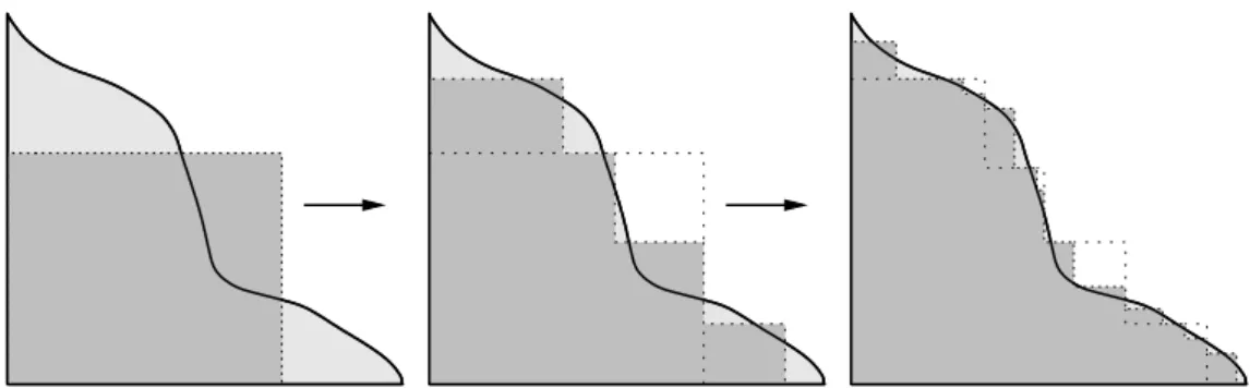
![Figure 4.8: Errors |P n −V H [S (0, 3)]| of the GAEP algorithm for the random vec- vec-tor having independent Pareto marginals with tail indexes θ 1 = 1 and θ 2 = 2.](https://thumb-us.123doks.com/thumbv2/123dok_us/8200198.2174158/47.892.204.778.488.895/figure-errors-algorithm-random-independent-pareto-marginals-indexes.webp)